Empirical model of VIX volatility and SPX variance

Received: 04-May-2024, Manuscript No. puljpam-24-7059; Editor assigned: 05-May-2024, Pre QC No. puljpam-24-7059 (PQ); Accepted Date: May 27, 2024; Reviewed: 06-May-2024 QC No. puljpam-24-7059 (Q); Revised: 08-May-2024, Manuscript No. puljpam-24-7059 (R); Published: 31-May-2024, DOI: 10.37532/2752- 8081.24.8(3).01-03

Citation: Lee PB. Empirical model of VIX volatility and SPX variance. J Pure Appl Math. 2024; 8(3):01-03.

This open-access article is distributed under the terms of the Creative Commons Attribution Non-Commercial License (CC BY-NC) (http://creativecommons.org/licenses/by-nc/4.0/), which permits reuse, distribution and reproduction of the article, provided that the original work is properly cited and the reuse is restricted to noncommercial purposes. For commercial reuse, contact reprints@pulsus.com

Abstract

We introduce a toy model for VIX futures dynamics using the Shifted-Lognormal Model (SLM) that does an excellent job of fitting VIX option prices with only two parameters. Then using the results of Roger Lee, who studied SLM models in detail, we propose a way to extrapolate VIX volatility surface which by construction is arbitrage free. Then, we derive analytical formula for forward variance in this model and relate risks of VIX volatility surface with that of SPX volatility surface by matching forward variance swaps results from both markets. This allows one to relate risk parameters between VIX and SPX volatility surface, namely we derive a nonlinear equation that relates VIX skew and SPX skew. This can be used for cross market hedging, arbitrage and enhanced risk monitoring.

Key Words

SPX volatility; SPX volatility surface; Nonlinear equation;Shifted-Lognormal Model

Introduction

The market participants are familiar that Shifted-Lognormal Model (SLM) does a reasonably good job fitting the VIX optionskew. We model each VIX future as a shifted log-normal process and by approximating variance swap to first order, we relate VIX volatility surface with that of SPX. Specifically, we show using the results of how changes in the VIX options skew impacts SPX options skew and vice versa [1]. This should be helpful as a toy model for risk management and to screen for any outsized mis-pricings between the SPX and VIX options markets.

In Lee gave upper limits of equity volatility for extreme log strikes [2]. Namely, he has shown that where k is log-moneyness. In fact, variance swap markets are well matched if one takes and most implied vol surface models extrapolate in this way such as the well-known SVI [2]. Similarly, using the results of the same author as, we can extrapolate how VIX volatility curve behaves for extreme log strikes in VIX in the SLM model [3]. This gives intuitive result that the probability of VIX being below certain extreme low value is zero which is defined by the floor parameter. For example, VIX spot has never closed below 9 according to Bloomberg data at least from year 1990, the earliest data is available.

Shifted-Lognormal Model (SLM)

In this section, we introduce the SLM model and review main results of relevant for our discussion. SLM model is simply the Black-Scholes model shifted by a constant parameter we call V_m which has natural interpretation as the VIX floor. The SLM stochastic process is given by

Where dW_t is Brownian motion. Taking V_m → 0, one recovers the standard Black-Scholes model, which has a flat vol surface by definition. Taking V_m to be positive makes the distribution shift to the right and the vol surface becomes positively skewed relative to Black-Scholes model in line with what is observed in the VIX options market. By defining V_t = (V_t - V_m), one readily obtains the Black-Scholes formula for calls and puts for a given strike K and expiry T. We ignore interest rates for simplicity in this paper but can be easily incorporated as an overall discount factor.

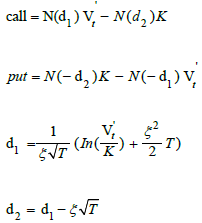
Here, ξ is the vol of vol parameter and V_t is the VIX future price at time t with expiry T. Figure 1 shows how this model does a good job of matching VIX options volatility surface for a given expiry (typically referred to as volatility slice or curve)

Figure 1: ξ = 335, V_m =13.8

Lee has done extensive work analyzing this model. For near limit, Lee has shown following Black-Scholes volatility formula in terms of ξ and V_m as a function of strike [1].

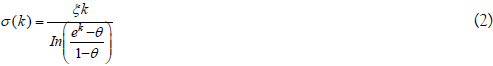
Where we define 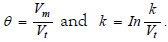For small values of k, Taylor expansion leads to

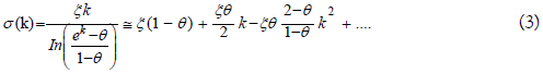
Taking the coefficients in the expansion, one has following descriptions of VIX vol surface near at the money

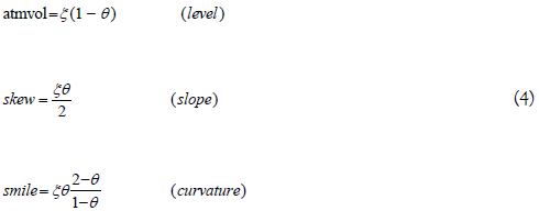
For extreme strikes, we have following results

Unlike equity vol surface, VIX volatility is bounded by vol of vol and is concave which is what is indeed observed in the VIX options market. Furthermore, any strike below the floor is worthless consistent with VIX options market where strikes below 10 are rarely quoted, whereas SPX strikes are regularly quoted up to $200 strike (less than 5% of current SPX spot price).

Strike extrapolation of VIX volatility surface

We have shown that VIX options curve behaves differently from that of equity options. In equities, implied volatility are extrapolated for extreme strikes as below

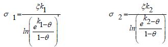
Where K is strike and F_t is the future price. Extrapolating at the upper limit given by matches the OTC variance swap market closely. However as seen above, VIX curve scales concave with log moneyness. In order to extrapolate strikes beyond listed strikes, we take the final 2 quoted strikes (or the last 2 liquid strikes) and solve for and to match the mid implied volatility levels at those strikes for both otm puts and otm calls separately. For example;

Dividing leads to

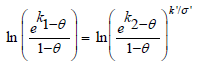
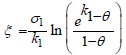
Where 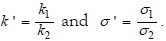and Once we solve for θ above (usingNewton’s method for example), one can solve for vol of vol as

We can then extrapolate the VIX curve using these matched parameters.

In Figure 2, we show an example of extrapolated VIX vol curve.

Figure 2: Extrapolated Jun’24 VIX vol curve as of 4/18/2024 2:30 pm

Forward variance and relation to SPX options

It is well known that SPX variance swap can be decomposed as integral sum of puts and calls with weights [4].

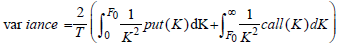
Where F₀ is the forward price. It is also possible to do similar calculation using VIX options to get the forward variance.

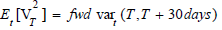
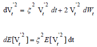
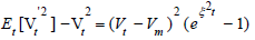
Here the calls are for VIX. However, in the SLM model, we can derive an analytical formula for the forward variance. Note that for VIX future V_t with expiry T one has-

Using Ito’s lemma and taking the expected value leads to

Now integrating the above with initial condition one obtains

Replacing 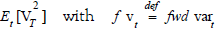with derived from the SPX options market yields following equation

Solving for the VIX future V_t, one has in the absence of arbitrage between the two markets,

Where This formula relates the SPX options market (fvt) to the VIX options market and acts as a toy model unifying the two markets.

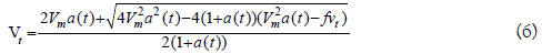
Next, we derive explicit relationship between the two markets using approximation for SPX variance swap expanding in log moneyness SPX skew. It is shown in that to the leading order [4].

Where we used the fact that SPX implied volatility surface can be parameterized as

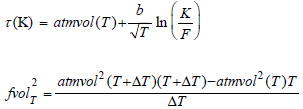
Δ is 30 calendar days as it is for VIX. Here we denote Black-Scholes implied volatility of SPX option as τ to distinguish from implied volatility of VIX options, and b is known as log moneyness skew for SPX. Market participants are aware that b is about constant across maturity and ranges between −0.2 to −0.3 in normal times. Plugging this approximation in equation (5), one has

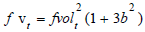
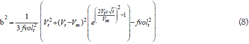
In practice, V_m is a slow-moving parameter relative to ξ. Finally using at the money results of equation (4) for VIX skew, one obtains the main result of this paper

where s is VIX options moneyness skew. This formula shows how VIX skew and SPX skew are related. In figure 3 we plot s(VIX skew) as a function of s(SPX skew) and see the relationship is close to linear. Intuitively, more negative SPX skew leads to steeper VIX skew for calls. We leave empirical study of this relationship for future work (Figure 3).

Figure 3: V_m = 11, V_t = 15, fvol = 13, t =1

References

1. Lee RW. The moment formula for implied volatility at extreme strikes, Mathematical Finance. Int J Math, Stat Fin Eco. 2004;14(3):469-80.

   [Google Scholar] [CrossRef]

2. Gatheral J, Jacquier A. Arbitrage-free SVI volatility surfaces. Quan Fin. 2014;14(1):59-71.

   [Google Scholar] [CrossRef]

3. Lee R, Wang D. Displaced lognormal volatility skews: analysis and applications to stochastic volatility simulations. Anna Fin. 2012;8:159-81.

   [Google Scholar]

4. Demeterfi K, Derman E, Kamal M, et al. More than you ever wanted to know about volatility swaps. Gol Sac quan strat resea not. 1999;41:1-56.

   [Google Scholar]