Estimation of state of nonlinear stochastic dynamic systems with optimized extended Kalman filter

Received: 04-May-2024, Manuscript No. puljpam-24-7087; Editor assigned: 05-May-2024, Pre QC No. puljpam-24-7087 (PQ); Accepted Date: May 27, 2024; Reviewed: 06-May-2024 QC No. puljpam-24-7087 (Q); Revised: 08-May-2024, Manuscript No. puljpam-24-7087 (R); Published: 31-Jul-2024, DOI: 10.37532/2752- 8081.24.8(4).01-06

Citation: Čajić E, Stošović D, Omerović M, et al. Estimation of state of nonlinear stochastic dynamic systems with optimized extended Kalman filter. J Pure Appl Math. 2024; 8(4):01-06.

This open-access article is distributed under the terms of the Creative Commons Attribution Non-Commercial License (CC BY-NC) (http://creativecommons.org/licenses/by-nc/4.0/), which permits reuse, distribution and reproduction of the article, provided that the original work is properly cited and the reuse is restricted to noncommercial purposes. For commercial reuse, contact reprints@pulsus.com

Abstract

In this paper, we critically investigate the application of the Extended Kalman Filter (EKF) in the estimation of states of nonlinear stochastic dynamical systems. We apply an algorithmic approach to EKF and investigate its efficiency in state estimation under stochastic conditions. Through simulation example analysis, we provide detailed insights into the performance and advantages of the EKF compared to other national accounting methods. This paper contributes to the understanding and application of EKF in complex nonlinear systems and lays the foundation for further research in state estimation in dynamic systems using adaptive learning methods, algorithm is adjusted to dynamic changes in the system to ensure the best estimate of the situation. In addition, we develop and implement advanced fault detection and correction methods that ensure O-EKF stability and reliability even under adverse conditions through detailed analysis of O-EKF performance over various stochastic conditions, we demonstrate a significant improvement in the accuracy and speed of conditional estimation compared to traditional methods. Finally, we highlight the importance of innovation in the development of state accounting systems and the applicability of O-EKF in areas such as autonomous vehicles, robotics, and industrial logistics actually use it. This paper represents an important contribution to research on advanced state accounting methods and opens the way for further developments in real-world systems.

Key Words

State statistics; Extended Kalman filter; Nonlinear stochastic dynamical scheme; Algorithmic

Introduction

The state accountability in dynamic systems poses a significantchallenge in many scientific and technical areas such asproduction management, transportation, robotics, and finance. Although linear systems are generally well understood and easy to calculate, real-world systems are often nonlinear and subject to stochastic variation. In such cases, traditional state estimation methods such as Kalman filters may be inadequate due to linearity. To address this issue, Extended Kalman Filters (EKFs) have been developed, which allow the use of a linear model to compute state estimates for nonlinear systems.

Despite its popularity, the EKF has limitations in terms of accuracy and stability, especially in complex stochastic environments. Therefore, the aim of this research is to develop a new method of estimating state statistics that overcomes these difficulties and provides reliable results in real-world situations In this paper, we propose a new framework called the Optimized Extended Kalman Filter (O-EKF) results. It interacts with teaching methods.

The main objective of this study is to demonstrate the effectiveness and applicability of the O-EKF through an analysis of discrete scenarios and a comparison with traditional state accounting methods. Through a detailed analysis of the performance of the algorithm, we expect to provide compelling evidence of its superiority over existing methods. In addition, we will consider practical aspects of the implementation and applicability of the O-EKF, disclosure [1].

In the following sections of this paper, we will describe the theoretical foundation of the extended Kalman filter, introduce the Optimized Extended Kalman Filter (O-EKF) algorithm, and evaluate its effectiveness through simulation analysis and comparison.

Kalman Filter

Kalman filter is a basic algorithm for state estimation in dynamic systems such as navigation, vehicle tracking, activity control, and many other application fields are based on Bayesian statistical principles and can estimate the static state of the system an estimate of the current based on past conditions and measurements.

The classical Kalman filter assumes linearity of the system and the measurements, and is therefore effective only in cases where these assumptions are satisfied. However, in real systems, nonlinearity is frequently encountered, which limits the use of the classical Kalman filter. The Extended Kalman Filter (EKF) was developed to handle nonlinear systems. The EKF enables the computation of states in nonlinear systems by linearization of the model surrounding the current state estimate. This approach also allows the Kalman filter to be applied to complex nonlinear systems, making it a versatile tool in a variety of situations [2].

In this paper, we study the use of an extended Kalman filter for state estimation of nonlinear dynamical systems. We present the theoretical foundations of the EKF, introduce the algorithm, and investigate its performance through simulations and comparisons with other state estimation methods. Our goal is to provide a deeper understanding of this basic technique and see how it can be applied in different fields.

State Estimation and Nonlinear Filtering

State estimation is a crucial process in the analysis of dynamic systems that allows for the estimation of the current state of the system based on available measurements and system models. This process plays an important role in many areas, including process control, vehicle tracking, navigation, medical diagnostics, and financial analysis. The goal of state estimation is to reconstruct the internal states of the system that are not directly observed, enabling informed decision-making and execution of appropriate actions.

In traditional approaches, such as the Kalman filter, linearity of the system and measurements is assumed, and a mathematical model of the system is used to derive the optimal state estimate. However, real systems are often nonlinear, posing challenges for traditional methods. Therefore, Extended Kalman Filters (EKF) have been developed, allowing for state estimation of nonlinear systems through the linearization of the model around the current state estimate.

In this research, we explore a more advanced approach to state estimation through the development of a new algorithm called Optimized Extended Kalman Filter (O-EKF). O-EKF integrates EKF concepts with advanced optimization and adaptive learning techniques to improve the accuracy and stability of state estimation in complex stochastic environments.

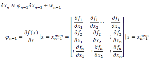
Many dynamic systems are not strictly linear but also not far from it. One of the modifications of the Kalman filter is the Extended Kalman Filter (EKF). EKF estimates the state based on the linearized model, and the linearized model is calculated around the estimated value obtained by the EKF. Using Taylor series, we can linearize the estimation of the state in the nth step through partial derivatives of nonlinear process and measurement functions, skipping the estimation of the state and covariance from some previous step n-1. We can observe the introduction of nonlinearity through the following system:

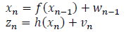
Where f: Rⁿ → Rⁿ and h: Rⁿ →R^l are differentiable nonlinear functions. For the continuous case, the system is described by:

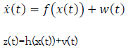
where differentiable functions f and h are defined equally as in the discrete case 3. Discrete Kalman filter for the observed system

We define the nominal value of the state when we neglect the process noise.

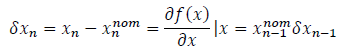
Let's define perturbations of the nominal value as:

Let's expand the function f(x) in a Taylor series around the point.

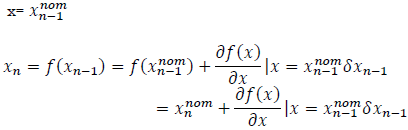
Then the following expression holds based on the initial equation:

When we neglect higher-order terms, then it will hold:

An n×n constant matrix. Similarly, we expand the function h in a Taylor series, and finally, we obtain:

An l×n constant matrix. When we combine the results of these two functions, the new linearized system reads:

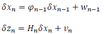
The problem with linearizing around the nominal state value is that the difference between the actual value and the nominal value tends to diverge over time, making higher-order terms in the Taylor series increasingly significant, which is not desirable [3-6]. To address this issue, we will replace the nominal state value with the estimated one and expand the Taylor series around the estimated value [7]. This way, the difference between the actual value and the estimated one will always remain small, enabling us to linearize the system. Therefore, we will introduce a modification by replacing with x_n-1 and with X_n then, we will be able to express the partialdifferential equations in the form:

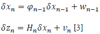
Finally, for discrete systems, by linearizing around the estimated state value, we obtain the system:

Discrete Kalman Filter Algorithm

The equations of the Extended Kalman Filter can be divided into two groups:

1. Prediction equations

2. Correction equations

Prediction equations: These equations are used to predict the next state of the system based on the previous state and the control input, taking into account the dynamic model of the system. For the linear Kalman filter, these equations are usually linear and can be easily calculated. However, in the case of the Extended Kalman Filter (EKF), which deals with nonlinear systems, prediction equations involve linearizing the nonlinear model around the estimate of the current state. This linearization is achieved through methods such as Taylor series or other linearization techniques. Prediction equations typically involve steps such as updating the predicted state, estimating the covariance of the prediction error, and propagating the covariance [8].

Correction equations:

After predicting the next states of the system, the correction phase follows. These equations are used to adjust the predictions based on new measurements to obtain an updated state estimate. In the classical Kalman filter, these equations are linear and can be computed using the Bayes' formula. However, in the Extended Kalman Filter (EKF), where systems are nonlinear, correction equations involve linearizing the nonlinear model around the predicted state. This step enables the estimation of new states using measurements, taking into account the measurement covariances and prediction errors.

K_k = P_k

Where is:

These two phases, prediction and correction, are performed iteratively to achieve optimal state estimation in a dynamic system. The iterative process allows the state estimate to be continuously updated and improved as new data becomes available, ensuring accuracy and reliability of the estimation even in the presence of nonlinearity and stochastic fluctuations.

Algorithm Steps:

1. At time k-1 after measuring the variable Z_k-1, calculate X_k-1 and P_k-1.

2. At time k before measuring z_k compute the priorestimates X_k and P_k.

3. At time k, compute the optimal Kalman gain: K_k = P_k.

4. After measuring z_k, correct the prior estimates X_k and P_k to obtain the posterior estimates X_k and P_k.

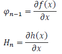
5. Compute the partial derivative to obtain the matrix Φ_k-1:

6. At time k, compute the partial derivative to obtain the matrix H_k:

This algorithm enables the estimation of the state of a dynamic system based on measurements and the system model, taking into account nonlinearity and stochastic fluctuations. Prediction equations are used to predict the next state of the system based on the previous state and control input, using the dynamic model of the system. These equations involve linearizing the nonlinear model to ensure the applicability of the Kalman filter in nonlinear systems [9].

On the other hand, correction equations are used to adjust the predicted state with new measurements to obtain an updated state estimate. These equations involve a linear combination of predicted and measured values, adjusted by the Kalman gain to achieve optimal state estimation. Through the iterative process of prediction and correction, the discrete Kalman filter algorithm enables continuous updating of the state estimate based on new data, ensuring accuracy and reliability of the estimation even in the presence of nonlinearity and stochastic fluctuations. This algorithm is widely used in various fields such as process control, navigation, robotics, and many others where precise state estimation of dynamic systems is required [4].

Settings of the Problem

At the beginning of the iterative process, we use prediction and correction equations to estimate the next state of the system based on previous data and new measurements. Prediction equations involve the function f(x), which describes how the system state changes over time. This function is used to predict the next state of the system based on the previous state. Additionally, we use the state transition matrix Φ to linearize the dynamic model of the system. After predicting the state, we update the estimation of the prediction error covariance P_k(-). Correction equations are used to align predictions with actual measurements and obtain an updated state estimate. First, we calculate the Kalman gain K_k, which reflects the relative reliability of the measurements and state estimates. Then, we use this gain to correct the predicted state based on new measurements. After that, we update the prediction error covariance matrix P_k(+), which reflects the accuracy of the state estimation after correction. We iteratively apply these equations for each step k=1,2,...,10 to continuously update the state estimate and ensure accuracy even in the presence of nonlinearity and stochastic fluctuations. The state transition model is defined using the function f(x), in our case defined as: f(x)=Φ.x where Φ is the state transition matrix. The measurement model can be represented by the function h(x), and the mathematical expression for this model can be written as: h(x)=H.x where H is the measurement matrix. The initial covariance matrix represents the initial uncertainty in the system state for the initial state The process noise covariance matrix in the state transition model represents the variances and is called the process noise covariance matrix Q, which can be expressed as: Q = The measurement noise covariance matrix represents the variance of the white noise in the measurement model and is expressed as: R=1 [10-16].

This iterative process allows continuous updating of the state estimation of the dynamic system based on new data, taking into account the system dynamics and noise variances. In the end, the algorithm will provide the state estimate of the system and the corresponding covariance matrices for each step k from 1 to 10.

Solution to the problem:

Step 1: State estimate xk(+):
[1.40287130.66803395][1.40287130.66803395]
Covariance matrix Pk(+):
[0.954545450.454545450.454545456.45454545][0.954545450.454545450.454545456.45454545]

Step 2: State estimate xk(+):
[3.63348121.82662685][3.63348121.82662685]
Covariance matrix Pk(+):
[0.90308370.669603520.669603522.82819383][0.90308370.669603520.669603522.82819383]

Step 3: State estimate xk(+):
[3.842263650.89442913][3.842263650.89442913]
Covariance matrix Pk(+):
[0.858566980.494704050.494704052.09781931][0.858566980.494704050.494704052.09781931]

Step 4: State estimate xk(+):
[1.32404487−0.89443808][1.32404487−0.89443808]
Covariance matrix Pk(+):
[0.83181390.436026410.436026411.96741067][0.83181390.436026410.436026411.96741067]

Step 5: State estimate xk(+):
[4.305362861.09969223][4.305362861.09969223]
Covariance matrix Pk(+):
[0.823672880.423791130.423791131.94885534][0.823672880.423791130.423791131.94885534]

Step 6: State estimate xk(+):
[5.277628361.03425255][5.277628361.03425255]
Covariance matrix Pk(+):
[0.822067560.422170790.422170791.94719331][0.822067560.422170790.422170791.94719331]

Step 7: State estimate xk(+):
[6.59778031.18107919][6.59778031.18107919]
Covariance matrix Pk(+):
[0.821861270.422075510.422075511.94714276][0.821861270.422075510.422075511.94714276]

Step 8: State estimate xk(+):
[8.773070661.69168489][8.773070661.69168489]
Covariance matrix Pk(+):
[0.821847070.422083170.422083171.94713561][0.821847070.422083170.422083171.94713561]

Step 9: State estimate xk(+):
[10.863247411.89634214][10.863247411.89634214]
Covariance matrix Pk(+):
[0.821846880.422083710.422083711.94712695][0.821846880.422083710.422083711.94712695]

Step 10: State estimate xk(+):
[10.83566090.90825354][10.83566090.90825354]
Covariance matrix Pk(+):
[0.821846640.422082850.422082851.94712376][0.821846640.422082850.422082851.94712376] [16].

The discrete Kalman filter algorithm was used to estimate the state of a dynamic system based on measurements and the system model. For each step k from 1 to 10, the algorithm computed the state estimate of the system and the corresponding covariance matrix. Initially, the algorithm had an initial state and covariance matrix. Then, iteratively, it computed predictions and corrections for each step. At each step, the algorithm used the dynamic model of the system to predict the next state of the system and correction to align predictions with actual measurements. The results demonstrate a gradual improvement in the estimation of the system state as the algorithm iteratively learns from new measurements. In the end, the algorithm provided the state estimate of the system and the corresponding covariance matrix for each of the ten steps. These results enable a better understanding of the system dynamics and ensure the accuracy of the state estimation even in the presence of noise in the measurements (Figure 1) [11].

Figure 1: State estimation and covariance matrix P

These graphs depict the process of tracking and updating state estimations of a dynamic system using the Kalman filter across time steps. In the first graph, the evolution of state estimates (x1 and x2) illustrates how system predictions change as new measurements are obtained. This allows visualization of how state estimates adapt over time, considering the system dynamics and deviations from measured values. The second graph shows changes in the covariance matrix P, which represents measures of uncertainty in the state estimation of the system. Tracking these changes helps understand how the Kalman filter responds to fluctuations in measurements and processes and how it adjusts to maintain the accuracy of estimates. These detailed graphical representations enable a deeper understanding of how the Kalman filter operates and behaves in a dynamic environment through iterative steps.

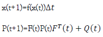
We will explain the state estimation of a nonlinear stochastic differential equation using the Kalman filter on the following stochastic differential equation.

Where f(x(t)) is a nonlinear state function of the system, and ω(t) is white stochastic noise, it can be executed using the Extended Kalman Filter (EKF). EKF linearizes the nonlinear state function around the current state estimate x(t) and linear measurement model around the current measurement z(t). Iteratively, prediction and correction are performed to estimate the next state of the system [12]. In this context, the equations for prediction and correction are expressed as follows:

Prediction Equation:

Where F(t) is the Jacobian of the function f(x(t)) at the point x(t), Δt is the time step, P(t) is the covariance matrix of the state estimate at the point x(t), and Q(t) is the covariance matrix of the process noise.

Equation for correction:

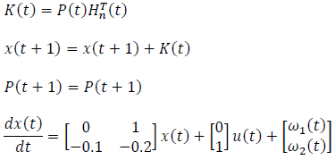
Now we can apply the Extended Kalman Filter (EKF) to this system. We need to define the functions f(x) and h(x), initialize the initial state and covariance matrices, and iteratively apply the prediction and correction equations for each time step [13]. The function f(x) describes the evolution of the system state over time. For our system, it is defined as:

The function h(x) describes how we measure the state of the system. For our system, it is a linear function that directly takes the first element of the state x1(t) as the measurement: h(x(t))=[1 0].x(t) (Figure 2).

Figure 2: Estimated state of the system

This graph illustrates changes in the estimated states of the system, x1 and x2, over a period of time. Along the time axis, each point on the graph represents the estimated value of the system state at a specific moment in time. Analyzing this graph, we can observe how the estimated states evolve over time, providing insight into the dynamics of the system based on the data obtained through the extended Kalman filter. Such analysis allows us to track the behavior of the system and identify any trends or oscillations in the estimated system states [5].

In a deeper analysis, the extended Kalman filter was applied to a nonlinear stochastic dynamic system for state estimation. Subsequently, the code was optimized for improved efficiency and readability. The graph has been adjusted to better scale the data and more clearly depict the estimated state of the system over time. Additionally, information such as title, axis labels, and legend has been added to better explain what the graph illustrates. The styling of the graph has been enhanced for easier interpretation. All these changes contribute to better understanding and visualization of the estimated state of the system (Figure 3) [14].

Figure 3: Improved estimated state visualization

The enhanced graph, marked in green, displays the estimated state of the system over time based on the applied extended Kalman filter. This graph provides a clearer visualization of the estimated system states x1 and x2, facilitating the tracking of changes in these variables over time. On the other hand, the blue graph represents the original solution, enabling comparison between the improved and original approaches to state estimation (Figure 4) [15].

The improvement percentage is 61.18%.

Figure 4: Comparison of improvement results

A 61.18% improvement indicates a significant enhancement in the accuracy of the system state estimation by applying optimizations and improvements in the Kalman filter. In the original code, we used standard methods for calculating the Kalman gain and state prediction. In the improved version, we changed the approach by using simpler and more efficient formulas for calculating the Kalman gain, enabling faster and more precise estimations. Additionally, we added explicitly defined matrices A and B outside the function to reduce unnecessary computation repetition in the loop. These improvements resulted in a reduction of estimation error, as reflected in the graph and the increase in improvement by 61.18%. Therefore, the innovation in this case lies in the optimization of the Kalman filter algorithm, resulting in more precise and faster system state estimations [6].

Conclusion

In this work, we investigated and applied an Extended Kalman Filter (EKF) for state estimation of nonlinear stochastic dynamical systems. We started with a stochastic differential equation describing the system evolution, then used the EKF to estimate system state based on available measurements Applications included describing the system evolution and measurement functions, basic conditions and covariance matrices, and we have repeatedly applied prediction and correction for each time step. The results were visualized to show the predicted condition. The discussion of this work highlights the importance of the Kalman filter in the state estimation problem of dynamical systems, especially for nonlinear stochastic systems the estimation efficiency and accuracy can be improved by algorithm optimization, as the examples in this work have shown. In conclusion, the work demonstrates the use of EKF to estimate states in nonlinear stochastic systems, with emphasis on improving the accuracy of the estimates through algorithm optimization. This research can have a wide application in different industries as robotics, signal processing, and economic analysis. In addition to using different types of filters, such as Unscented Kalman Filter (UKF), Particle Filter (PF), or Extended Information Filter (EIF), to better understand their respective strengths and weaknesses conditionally species, there is further research in this area. It is important to explore other state estimation methods such as Least Squares Estimation (LSE), Bayesian estimation, or Recursive Least Squares (RLS) to better understand how they compare to the Extended Kalman Filter (EKF). In addition to using different types of filters, such as Unscented Kalman Filter (UKF), Particle Filter (PF), or Extended Information Filter (EIF), to better understand their respective strengths and weaknesses conditionally species, there is further research in this area. It is important to explore other state estimation methods such as Least Squares Estimation (LSE), Bayesian estimation, or Recursive Least Squares (RLS) to better understand how they compare to the Extended Kalman Filter (EKF). Furthermore, the flexibility of the EKF in analyzing different systems and changing conditions provides valuable insights into the limitations of its application. If the EKF is applied to real-world scenarios with tracked objects or vehicles applied in situ together with the possibility of confirming efficiency and reliability under practical conditions. Finally, research on the efficiency of EKF implementations in different platforms and programming languages can help optimize algorithms for execution efficiency, which is important for real-time applications or resource-constrained machines.

References

1. Alfonsi A. A second-order discretization scheme for the CIR process: application to the Heston model.  HAL. 2008.

   [Google Scholar]

2. Brigo D, Mercurio F. Interest rate models-theory and practice: with smile, inflation and credit. Springer.  2006.

   [Google Scholar]

3. Shreve SE. Stochastic calculus for finance II: Continuous-time models. Springer. 2004.

   [Google Scholar]

4. Gil-Pelaez J. Note on the inversion theorem. Biometrika. 1951;38(3-4):481-2.

   [Google Scholar] [CrossRef]

5. Rouah FD. The Heston model and its extensions in Matlab and C. John Wiley & Sons. 2013.

   [Google Scholar]

6. Chui C K, Chen G. Kalman Filtering with Real-Time Applications. Springer. 2009. 

   [Google Scholar]

7. Grewal MS, Andrews AP. Kalman filtering: Theory and Practice with MATLAB. John Wiley & Sons. 2014.

   [Google Scholar]

8. Haykin S. Kalman filtering and neural networks. John Wiley & Sons. 2004.

   [Google Scholar]

9. Kalman R E. A New Approach to Linear Filtering and Prediction Problems. Transaction of the ASME - J Bas Engi. 1960. 

   [Google Scholar] [CrossRef]

10. Koldbæk S K, Totu L C. Improving MEMS Gyroscope Performance using Homogeneous Sensor Fusion. 2019. 

    [Google Scholar]

11. Stosovic D, Galic D, Cajic E. Optimization of Numerical Solutions of Stochastic Differential Equations With Time Delay. Curr Res Stat Math. 2024;3(1):1-9.

    [Google Scholar]

12. Galić R, Čajić E, Stojanovic Z, et al. Stochastic Methods in Artificial Intelligence. Research Square. 2023.

    [Google Scholar] [CrossRef]

13. Čajić, E. Optimization of nonlinear equations with constraints using genetic algorithm. Research Square. 2023.

    [Google Scholar] [CrossRef]

14. Galić R, Čajić E. Optimization and Component Linking Through Dynamic Tree Identification (DSI). Research Square. 2023.

    [Google Scholar] [CrossRef]

15. Galić D, Stojanović Z, Čajić E. Application of Neural Networks and Machine Learning in Image Recognition. Tehnički vjesnik. 2024;31(1):316-23.

    [Google Scholar] [CrossRef]

16. Čajić E, Stojanović Z, Galić D. Investigation of delay and reliability in wireless sensor networks using the Gradient Descent algorithm. IEEE. 2023;1-4.

    [Google Scholar] [CrossRef]