Existence and Smoothness of Solutions to the Navier-Stokes Equations Using Fourier Series Representation

Received: 04-May-2024, Manuscript No. puljpam-24-7080; Editor assigned: 05-May-2024, Pre QC No. puljpam-24-7080 (PQ); Accepted Date: Jun 20, 2024; Reviewed: 16-May-2024 QC No. puljpam-24-7080 (Q); Revised: 28-May-2024, Manuscript No. puljpam-24-7080 (R); Published: 31-Jul-2024, DOI: 10.37532/2752- 8081.24.8(4).01-02

Citation: Petros BA. Existence and smoothness of solutions to the navier-stokes equations using fourier series representation. J Pure Appl Math. 2024; 8(4):01-02.

This open-access article is distributed under the terms of the Creative Commons Attribution Non-Commercial License (CC BY-NC) (http://creativecommons.org/licenses/by-nc/4.0/), which permits reuse, distribution and reproduction of the article, provided that the original work is properly cited and the reuse is restricted to noncommercial purposes. For commercial reuse, contact reprints@pulsus.com

Abstract

We propose an analytic solution to the Navier-Stokes equations based on periodic initial velocity vector fields. By leveraging the Fourier series representation of periodic functions, we express the velocity field as Fourier series expansions and analyze their evolution over time. This approach provides insight into the existence and smoothness of solutions under specific periodic conditions.

Key Words

Analytic solution; Navier-stokes; Periodic conditions; Electromagnetic interaction; Thermal phenomena

Introduction

The navier-stokes equations describe the motion of fluidsubstances and are fundamental in fluid dynamics. The existence and smoothness of solutions to these equations, particularly in three dimensions, remains an open problem. In this paper, we investigate an analytic solution based on periodic initial conditions and Fourier series representations to address the existence and smoothness problem.

Periodic function representation

For a, b, c real constants, consider a unit vector A as a period vector satisfying the normalization condition be:

A= ia + jb + kc

||A|| = 1⇒ a² + b² + c² = 1

For x, y, z real variables, let the position vector r be:

r = ix + iy + kz

The dot product of A and r is given by:

A·r = ax + by + cz

For incompressible viscous fluids in the absence of external forces, the navier- stokes equations take the form:

where u is the velocity vector field, p is the pressure, ν is the viscosity, and ∇ is the gradient operator.

Initial velocity vector field

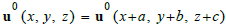
Let the initial velocity vector u⁰(x, y, z) be periodic, represented as:

This can be expressed using a Fourier series in terms of the dot product of a unitary period vector A and position vector r:

The derivation of Fourier coefficients involves integrating the product of the initial velocity vector field and trigonometric functions over the domain. By satisfying orthogonality conditions, we compute the coefficients analytically, ensuring the accuracy and efficiency of the solution.

To find the coefficients a₀, a_n, and b_n, we use the orthogonality properties of sine and cosine functions. The coefficient a₀ is the average value of the function over the domain and is solved using equation 4.

To find a_n, we multiply u⁰(x, y, z) by cos (2nπ(A · r)) and integrate over the domain and use equation in 4:

To find b_n, we multiply u⁰(x, y, z) by sin (2nπ(A · r)) and integrateover the domain and use equation 4.

Proposed solution for velocity field

We propose an analytic solution for the Navier-Stokes equations given the periodic initial velocity vector field. The velocity field u(x, y, z, t) can be expressed as:

Pressure field

The scalar pressure solution from the initial condition and proposed velocity vector field solution is:

Proof of existence and smoothness

Existence of solutions: The existence of solutions can be demonstrated by substituting the proposed forms of U and p into the Navier-Stokes equations and showing that these forms satisfy the equations under given initial conditions.

Continuity equation: Divergence of equation (8) for g = A · r + k(t) is simplified to

Using divergence free condition of equation (2) and equation (13) we can get.