Extension of Newton’s universal law of gravitation across space and time domains

Received: 07-Nov-2024, Manuscript No. PULJMAP-24-6632; Editor assigned: 12-Nov-2024, Pre QC No. PULJMAP-24-6632 (PQ); Accepted Date: Dec 23, 2024; Reviewed: 26-Nov-2024 QC No. PULJMAP-24-6632; Revised: 01-Nov-2024, Manuscript No. PULJMAP-24-6632 (R); Published: 29-Dec-2024, DOI: 10.37532/puljmap.2024.7(4);01-10.

Citation: Yalcin A. Extension of Newton��?���¢??s universal law of gravitation across space and time domains. J Mod Appl Phys 2024;7(4):1-11.

This open-access article is distributed under the terms of the Creative Commons Attribution Non-Commercial License (CC BY-NC) (http://creativecommons.org/licenses/by-nc/4.0/), which permits reuse, distribution and reproduction of the article, provided that the original work is properly cited and the reuse is restricted to noncommercial purposes. For commercial reuse, contact reprints@pulsus.com

Abstract

Newton’s universal law of gravitation has not lost any of its value for centuries. Despite some constraints, this law is indispensable in many applications due to its simplicity, clarity and high reliability. The new theory outlined in this article eliminates the constraints of the law, updates it to include the process of interaction in space and time domains and gives it a real universal character. The theory accomplishes this by incorporating the kinetic energies of the masses into the interaction process. As all quantities in the equations in the new theory are expressed in terms of Newtonian multipliers, it is a generalized form of Newton’s gravity law. This guarantees the simplicity and extraordinary reliability, not only in a stationary universe but also, in a continuously changing dynamic universe by making the equations valid, in all distances from atomic scale to cosmological scale and in all velocities from zero to the light velocity. This article derives the force relations based on outlined concrete observations and provides phase plot diagrams for two extreme situations and interprets them. At the end of the article, a list of potential solutions suggested by the theory is given for today’s fundamental physics problems. The most appropriate expressions for describing the theory are its field relative and dialectical characters. The theory can be verified with hundreds of examples. With phase plane diagrams that validate the theory in its fundamental aspects, only the solution of the Flyby Anomaly is exemplified to restrict the article to an acceptable length. The last example of a binary stars provides clues as to how we should handle interaction at the atomic level.

Keywords

Newton’s universal law of gravitation; Indispensable; Stationary universe; Cosmological scale

Introduction

Newton’s universal law of gravitation, which is also known as the inverse square law, is expressed by the following formula (Spiegel):

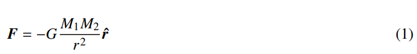
where F is the attraction force of two objects, g is the universal gravitational constant, M1 and M2 are the masses of the interacting objects, r is the distance between the masses and rˆ is the unit vector towards the point where the second object is located. The minus sign indicates that the gravitational force F and the unit vector rˆ are oriented in opposite directions [1].

The law is universal as it is valid on earth, the solar system and the universe. However, the law is valid at a fixed distance r and for that moment only. As the force causes a distance change for a time duration of the two bodies, the equation does not include the distance change and time information, (Zee) i.e., it does not involve the process of interaction. Therefore, the equation is reliable only if the distance between the two bodies does not change in some way as a result of the interaction. If a movement of an object on earth makes only negligible changes relative to the radius of earth or if an object that moves around a gravitational field source maintains a constant distance to the source mass, as in artificial satellites and planets, then Newton’s gravitation law yields extremely reliable results. Thus, the law is indispensable [2].

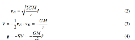
After Michael Faraday’s first insertion of the field concept in physics (Weinberg), the gravitational potential field was extensively employed in the interaction of masses in nature. Accordingly, each point in the domain of a mass can be depicted in three different field magnitudes and each field magnitude can be derived from the other field: Escape Velocity (vE), gravitational potential (V) and gravitational or force field (g). These fields are expressed as (Javid):

Field theory offers new possibilities for understanding nature. Based on this, Gauss redefines the gravity phenomenon known as Gauss’s law of gravitation which is expressed in integral form as follows (moody):

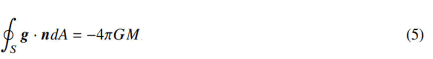
where the left side of the equation is flux (Stewart) of the gravitation field on a closed surface containing the source mass M, n is normal unit vector on the closed surface pointing outwards and dA is infinitesimal small area on the surface [3].

Gauss’s law is equivalent to Newton’s law of gravitation, but it has a more flexible use, for example the "spherically unsymmetrical" gravitational field of a voluminous and non-homogeneous mass can be calculated more accurately.

In our opinion, with the field concept, the remote effect problem of Newton’s law of gravity is solved. A force relationship does not directly exist between two objects but between the potential field created by one mass and the other mass. However, the base problem in Newtonian dynamics remains. The new problem is to identify the potential field and determine how fast it is created. The field concept does not change the inverse square structure of the theory hence does preserve the same constrains.

The Mond theory proposes a modification of Newton’s second law of motion to provide a solution to the speed-distance mismatch in spiral galaxies as an alternative to the assumption of black matter (Milgrom). Although different versions of the Mond theory exist (Milgrom), the results are not been fully compatible with the observations.

Kinetic energies in interaction

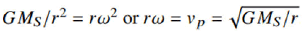
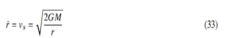
The starting point of the new field relative theory is extremely simple. The interaction occurs between the potential field energy created by the effective object (field source) and an affected object. Thus, the kinetic energy of the objects should have a role in the interaction. We can observe the accuracy of this approach with two very simple and well-known experiments. In the first example, the affected object will move in a radial direction with respect to the effective object and in the second example, both objects will maintain a specific distance between each other. In both instances, one of the masses of the objects (effective object) is incomparably larger than the other mass of the object, which is the most reliable application of the Newton’s law of gravity. For the first example, Figure 1 depicts the behavior of a stone that is vertically thrown from the ground with two different initial velocities. The larger is the initial velocity of the stone, the higher it climbs. As the stone ascends, both its velocity and the escape velocity of earth at this point decrease. The distance (γ) from the center of Earth determines the decrease in velocities. Equations 2 and 4 indicate that the velocity of the stone and the escape velocity decrease in the form of

respectively. As the stone decelerates at a faster rate, its upward velocity at the highest point will be zero and it will start free fall. Figure 1 shows all velocities of the stone along the route that it follows (green arrows), the escape velocities at this point (purple arrows) and their differences (red arrows). This condition applies where the initial velocity of the stone on the left side of Figure 1 is smaller than the escape velocity on earth’s surface. On the right side of Figure 1, the initial velocity of the stone that is thrown upward is equal to the escape velocity at the ground. In this case, the stone will not feel earth’s escape velocity and consequently, the gravitational force; thus, it will maintain its upward velocity. In this case, as the escape velocity decreases while the stone rises, the difference between the two velocities will continue to increase. Therefore, the upward velocity of the stone should increase. In the beginning, the stone maintains its unique velocity, while the resistance (gravitational force) that attempts to pull it down is reduced. In this case too, Figure 1 shows all the stone and escape velocities and their differences [4].

Figure 1: Vertical launch path of a stone with various initial velocities. The stone, in any case, always follows the increasing perceived (relative) escape velocities (red arrows).

Figure 2: Effects of various satellite velocities. If the relative escape velocity (satellite orbital velocity minus escape velocity) is constant, then the satellite is in equilibrium in the orbit. If the satellite velocity is less than the orbit velocity, then the satellite approaches the earth and the relative escape velocity negatively increases. If the satellite speed is greater than the orbital speed, the opposite happens.

• If the object does not detect the escape velocity (if the velocity of the object is equal to the escape velocity) or if it detects a fixed magnitude escape velocity, the object will maintain its velocity magnitude (kinetic energy). In this case, the interaction between the two bodies is a balanced interaction.
• If the escape velocity perceived by the object negatively increases (towards the source body), the object will approach the escape velocity field source. The interaction assumes the form of attraction.

If the escape velocity perceived by the object positively increases (away from the source body) the object will move away from the escape velocity field source. The interaction assumes the form of repulsion.

Materials and Methods

The notion of interaction in the form of repulsion may be unpleasant to some people. However, this notion is a distinguishing feature of the theory and is extremely logical. Figures 1 and 2 show that the interaction is the power conflict between the field potential energy and the object kinetic energy [6]. These energies are both the cause and the result of the interaction as not only the effective potential field in the interaction but also the kinetic energy of the affected object is decisive and the interaction process will change both magnitudes as results. This type of process is dialectical aspect of the interaction. As shown in Figures 1 and 2, if no balanced interaction exists, the difference between the two energies will always increase. This finding is logical as interaction creates a force that will give the affected object more energy. If the total kinetic energy of the object (object velocity) remains below the field potential energy (escape velocity) in the process, the attraction interaction will be effective. If the kinetic energy of the object is greater than the field potential energy and the field potential energy decreases during interaction, the repulsive interaction will be inevitable [7].

Escape velocity versus gravitational potential

The potential energy field of a mass and the escape velocity are two different aspects of the same physical phenomenon. Therefore, mathematically and physically, both aspects are equally important. Using the escape velocity field instead of the scalar gravitational potential field in the interaction has many other advantages, which can be summarized as follows:

• The velocity field is a tangible field that can be more easily understood using our mental perception than the abstract gravitational potential field.
• As previously described, the perceived (relative) velocity field can be easily defined between objects and field velocities to implement the true relativity concept in the interaction.
• A scalar gravitational potential, which specifies a point in a field that corresponds to an infinite number of velocity quantities that have equal magnitudes but are oriented in different directions. Therefore, a potential field can logically emerge due to a velocity field, i.e., equation 3 can be derived from equation 2 but the reverse cannot be true. This finding shows that the escape velocity has a considerably greater priority to describe the nature than the potential field. The escape velocity is not the result of the potential field but its cause.
• Mathematically and physically, a vector quantity for a point in the effective field is more informative than a scalar quantity. Therefore, if a scalar quantity is employed instead of a vector quantity, a loss of information is inevitable. For instance, repulsive effect of the mass interaction cannot be recognized.
• The effect of the spin velocities of interacting bodies can easily be included in the interaction for completeness. By performing this action, the interaction equation attains a true universal nature, i.e., it becomes valid in both macrocosms and microcosms.
• The concept of field velocities surprisingly reveals that the space behaves as an uncompressed fluid with considerably low density, which solves the mystery associated with the gravitational interaction. The Bernoulli principle (Bachelor) can be assumed to be valid in space and the varying field velocities define inversely varying pressure mediums for force relations. The gravitational attraction exists because masses exhibit higher velocity fields (lower-pressure mediums) at close distances and a force exerted from higher-pressure mediums to lower-pressure mediums is inevitable.

The Bernoulli principle is emphasized in this paper only for the understanding of the interaction mechanism. Use of the velocity field does not hinder the use of the gravitational potential to determine the force relations between objects. The conventional approach to derive a force relation starting from the potential field is safe and universally accepted and its validity has been confirmed. However, the new theory uses the dynamic potential field perceived by the affected object instead of the conventional gravitation potential.

Inertial frames and mass size ratio

We need to remember a topic of Newtonian mechanics, which will help us to understand the role of mass magnitudes in the interaction. Figure 3 depicts a two-body system in which all parameters are necessary for an interaction process with reference to the centroid. Here, the two bodies are only under the influence of each other’s interaction force. Calculations with reference to the centroird (inertial frame) will be accurate and reliable. Here, γ=γ₂-γ₁ is the distance vector between the two bodies and ν_R=ν₂−ν₁ is the relative velocity. Since 0 is the centroid, M₁γ₁+M₂γ₂=0 and M₁ν₁ + M₂ν₂=0 can be written [8].

Accordingly, the position vectors and the velocity of each object are expressed in terms of the distance vector and the relative velocity as follows:

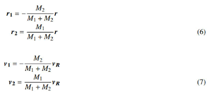
If M₁=M₂, the centroid will be in the middle of the line that joins the objects and their position and velocity vector magnitudes will be the same; however, their directions will be opposite, i.e., γ₁=-γ₁=-γ/2 and γ₁=ν₁=- ν₂=ν_R/2. If one object is extraordinarily large compared with the other object, the centroid will be almost in the same location as the larger object and the position vector and the velocity of the other object will be the same as the distance vector and the relative velocity, i.e., γ₂=γ, γ₁=0 and ν_R=ν₁=0.

Field relative equations

The mathematics of the field relative theory has a very simple logic: It does not directly use the gravitational potential derived from the escape velocity Journal of Modern and Applied Physics J Mod Appl Phys Vol.7 No.4 2024 3 but uses the relative field potential derived from the perceived escape velocity by the affected object (Figure 3) [9].

Figure 3: Two-body system parameters with reference to the centroid. Here, ν₁, ν₂ are position vectors and ν_E1, ν_E2 are object velocities, escape velocities and spin velocities of ω₁, ω₂ masses respectively.

To complete the picture, we need to add the field effect of the spin velocity of the celestial bodies to the escape velocity. The rotation of the celestial bodies around their axes (spin) is general, with the exception of some special cases. As a celestial body rotates around its axis, the escape velocity field in its domain will also rotate. Otherwise, constructing earth’s gravity map with remote sensing with GRACE (NASA) and GOCE projects would not be meaningful. If a celestial body has a spin velocity, a second field velocity component is expressed in the following formula in addition to the escape velocity of each point in the domain:

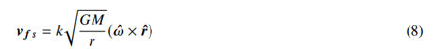
where, ν_fs is the azimuthal component of the field velocity, ωˆ is the unit vector in the rotational axis direction of the source body and k is the scaling factor, which is the ratio of the tangent velocity component of the field rotation at the equator of the source body to the escape velocity. The scaling factor is the value of the tangential rotation velocity in the equator plane in terms of escape velocity at that point. The rotating velocity field distribution will assume the horn-torus form (Weisstein), i.e., it will have the largest value in the equatorial plane and zero value along the axis of rotation [10]. In rocky-type planets, since each point of the planet has the same angular velocity, the scaling factor can be calculated with the following formula:

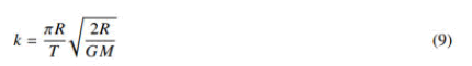
where, R is the radius of the planet and T is the spin period. For celestial bodies with different angular velocities, such as gas giant planets and the sun, the scaling factor k can only be obtained by experimental methods. For celestial bodies, k has a very small value and is negligible for most applications. For example, k=0.0415 for earth and 0.003 for the Sun based on the rotation that appears at the equator. Given the average rotation time of the Sun as a whole, the real value will be considerably smaller. If a celestial body rotates around its axis, the total field velocity ν_fT will be equal to the sum of the escape and spin velocities:

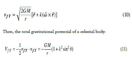
Where Θ is the angle between ωˆ and γ. Thus, θ=90° is the equatorial plane of the rotating celestial body. If we compare this equation with equation 3, the mass of a rotating object will appear larger in the equatorial plane. Thus,

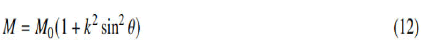
where M₀ is the rest mass of the celestial body without spin motion. Thus, an energy condensation exists in the equatorial plane of a rotating object. Accordingly, considering the gradient operation in spherical coordinates, the acceleration field of an object:

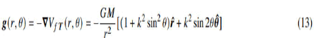
Both the total potential and the acceleration fields are expressed in Newtonian multipliers. The acceleration field in a rotating object is not spherically symmetrical. The radial acceleration is larger in the equatorial plane and the acceleration has a polar component. This component suppresses the objects in the domain to the equatorial plane. Since the potential field of a rotating celestial body is not spherically symmetrical and due to the components other than the radial acceleration, we will refer to the fields as potential and acceleration fields instead of gravitational potential and gravitational fields [11].

Conclusion 1: If the source mass that forms the potential field has a spin motion, global clustering cannot occur and flat clustering is mandatory. Spiral galaxies, the solar system and the rings of Saturn are undeniable observations that confirm this result.

Conclusion 2: The faster is the spin of the main element in the center of a spiral galaxy system, i.e., a black hole the greater is its perceived mass in the equator region. The radial acceleration component in the equator region will be substantially larger than the Newtonian gravitational acceleration, i.e., the objects in the equatorial plane have orbital velocities that are greater than those prescribed by Newton’s gravitational law.

Interaction

We have observed that how each object in the interaction of two bodies perceives the escape velocity of the other is decisive. As shown in Figure 3, how each object perceives the total velocity field formed by the other object can be expressed as:

Since the interaction between two masses is in the form of a force applied by the velocity field created by one to the other, the forces exerted by the masses on each other are independent of each other.

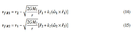
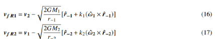
Here, we have to address a very basic and serious problem. I think that this problem is the most fundamental problem in traditional physics on every scale. Most of the time, Figure 3 and equations 14 and 15 do not refer to reality in nature. Theoretically, to write these equations, all object and field velocities must be synchronized, i.e., should express simultaneous velocities. However, any two objects that interact in nature are located at different points in space. The distance between them is very small on an atomic scale, but it is millions and even billions of kilometres in macrocosms. Regardless of the distance, in theory, mathematically no obstacle to simultaneously evaluating the field and object velocities of the two objects exists. However, equations 14 establish a link between the object velocity and the escape velocity created by the other object. For this bond to express a reality, regardless of the distance, the escape velocity must instantaneously follow its remote source (infinitely fast effect velocity). However, this is not possible; even the theory of general relativity states that the speed at which a source can create its space-time curvature cannot exceed the speed of light. Thus, neither Figure 3 nor the equations 14 and 15 have real equivalents in nature. In order for these equations to be valid, we have to consider the time it takes for the field velocities to reach the interaction points [12]. For this, suppose we will calculate the relative field velocities at time t0. Let t-1 and t-2 be the time intervals which take for the field velocities to arrive from M1 to M2 and from M2 to M1, respectively. In this case, we can write the relative velocities as follows:

Here γ_-1 is the distance between M₁ at t(-1)=t0-t₋₁ and M₂ at t0 and γ₋₂ is the distance between M₂ at t(-2)= t₀-t₋₂ and M₁ at time t₀. According to the theory, since the field velocity is equal to the escape velocity, that is, if the masses are different in size, γ₋₁ will be different from γ₋₂ since the two field velocities are different.

However, equation 14 will be valid under only one condition. If M₁>>M₂, then ν₁=0 according to Figure 3 and equation 7. In other words, M₁ will not be affected by the force interaction and will maintain its position 7 continuously. In this case, the velocity field of M₁ will also remain stationary in the radial direction. Equation 14 will always accurately describe the velocity field of M₁ regardless of time. This is obviously equivalent to the effect velocity of the field of M₁ being infinite [13]. In this case, the relative potential field consisting of the relative velocity field of M₁ is:

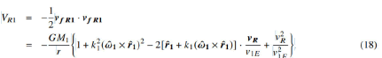
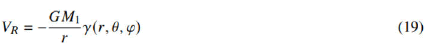
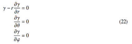
Here ν_1E is the escape velocity of M₁ at the point where M₂ is. In these conditions, that is, in the case of M₁>>M₂, the force exerted by the velocity field of M₂ on M₁ can be neglected. As can be seen, Newton’s spherically symmetric gravitational field is the multiplier of the relative gravitational field perceived by M₂. The new multiplier in the expression will be called the "field distribution factor" γ. The effective gravitational potential is no longer spherically symmetrical due to the spin velocity of M₁ and the kinetic energy of M₂ and is dependent on all three axes (γ,θ,∂) in spherical coordinates. Therefore, the relative potential field can be written as:

Accordingly, the acceleration of M₂ due to the effective field of M₁ in its domain can be written in spherical coordinates as follows:

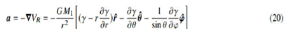
It should be noted that this is not the acceleration of the field, but the acceleration of the affected object in the field. Because the acceleration value was created from the field velocity perceived by the object. The mass M₁ will create not only a central force in its effective field but also polar and lateral force components. These components in terms of the Newtonian multiplier are:

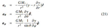
The following results can be clearly stated from these equations:

In the most general sense, the force interaction between the masses is not limited to gravity. There will also be lateral and polar components of the interaction due to the rotation of the velocity field source around its own axis [14].

If the rotational velocity of the source mass and the linear velocity of the affected mass are not taken into account, then γ=1 and the potential field will be reduced to the Newtonian gravitational potential. In this case, the interaction will only create a central gravitational force.

The multiplier in the radial component may be negative, zero or positive.

• If this multiplier is zero, no radial force relationship exists between the two masses. This corresponds a balanced force relationship, as in the sun-planet example. • A negative multiplier indicates that the mass interaction is in the form of repulsion. In other words, mass repulsion as well as gravity in general is part of the interaction under certain conditions. This repulsive form of interaction provides coherent solutions to observations of gravitational redshift, "Pioneer anomaly" (blueshift of light approaching the solar system) and even to observations of the acceleration and expansion of the universe. These three phenomena are likely to be the normal behavior exhibited when the velocity of the affected object is greater than the escape velocity of the source mass. The dark energy assumption should be seriously questioned. • If the multiplier is negative, the interaction will be in the form of gravity, which is the most familiar application.

If the two masses are in equilibrium in terms of the force relations, all three acceleration components will be zero and the following equations will apply:

Zero acceleration in all three axes implies that the axial velocities are not only zero but at a constant velocity. This condition determines the stable trajectory of the affected body around the velocity field source.

The source of flat clustering in nature is the polar component of acceleration. The spiral galaxies have a flat structure due to the high-speed rotating black holes in their centres. Similarly, the planets are clustered in the equatorial plane of the Sun due to the rotation of the Sun around its axis. Saturn’s high rotational speed renders the equatorial plane energyintensive and therefore, beautiful rings are formed [15].

The source of the lateral component of acceleration is the spin motion of the source mass, which explains why all stars in spiral galaxies, all planets and the Sun spin and Saturn and its rings rotate in the same direction. The deviation of the axis of Mercury is also attributed to this lateral acceleration component and applies to all planets. However, this effect increases as you approach the sun. The larger is the orbit eccentricity, the more visible is the axial deflection. No axial deviation exists in the full circular orbit as the axis of the orbit is meaningless. Therefore, this slight deviation can only be observed in the orbit of Mercury. The lateral component of the acceleration also indicates that it is dragging the affected bodies. For this reason, it is necessary to take this drift velocity into account in the orbital velocities of stars and planets. Moreover, the linear velocities (kinetic energies) of inner stars in galaxies are never taken into account in conventional physics. Since these stars will drag their velocity fields with them, all stars are also under the effect of others’ drift velocity, which is not taken into account. This fact may disprove the dark matter hypothesis [16].

Planets in orbit

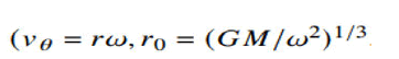
Since mass-size ratios are 0.001 or less in the sun-planet interaction and the spin scaling factor k for the Sun is also very small, the field dispersion factor γ in equation 18 can be expressed very approximately as:

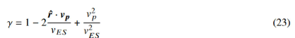
This expression will define a complete reality because the sun is almost stationary. In the formula, ν_ES is the Sun’s escape velocity at the planet location and νp is the planet velocity. In a heliocentric spherical coordinate system with the planet’s orbit as the horizontal plane, we can express the planet velocity in the position vector γ as follows:

Considering the escape velocity of the Sun, from equations 21, 23 and 24 the radial acceleration a_r of the planet is as follows:

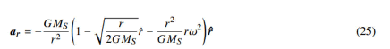
where ω=φ is the angular velocity of the planet in orbit. If the planet moves in a circular orbit, then a_r=0. The parentheses in equation 25 must be zero. In this case, since γ=0 in a full circular orbit, the following expression should be zero:

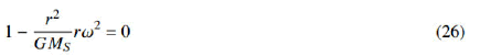
This equation is another expression of

We are quite familiar with these equations from Newtonian celestial mechanics. The first expression yields the equality of the centripetal acceleration to the centrifugal acceleration and the second expression yields the average velocity in the planet’s orbit. In general, we can express equation 25 as follows:

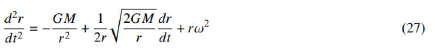
Newtonian mechanics includes only the first term on the right in this equation.

The other two terms refer to the planet and field velocities and are specific to the new theory. We have simplified the equation by assuming that the angular velocity of the planet in orbit is constant. This equation is a quadratic non linear differential equation that contains all information about the movement of the planet in orbit; unfortunately, it has not an explicit solution [17]. However, we can apply our mathematical knowledge to make some conclusions. First, the equation can be reduced to two firstorder equations as:

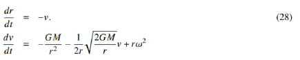
where ν is the planet speed on the orbit. Since the velocity of the planet decreases with an increase in the distance from the Sun, the speed variable is negative in the first equation. These two equations form a typical nonlinear autonomous differential equation system (Jordan). To work on it, we had to apply non-dimensionalization and a scaling process to obtain a more general mathematical expression (Perez). We will employ the following transformation and scaling values:

Thus, the nonlinear autonomous system of equations will be expressed as follows:

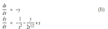
In this equation, x represents the distance between two interacting objects and y represents the speed of the affected object. At a stable point, both variables must be constant for zero derivatives. Thus, the right side of the two equations must be zero at the same time. If this condition is satisfied, this point is referred to as a critical point. In our system, the critical point is (x₀=1, y₀=0). This point represents the point in real nature.

i.e., the average velocity of the planet in the orbit and the distance between the two objects. The non-dimensionalization and scaling process shifted the average velocity of the planet to zero point. Variable y determines increasing and decreasing velocities around average value on the orbit. Whether this point is balanced or unbalanced can be easily determined by the phase plane plots. At this critical point, the Jacobian matrix is created to linearise the non-linear system and the eigenvalues of this matrix are:

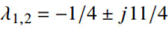
These eigenvalues (two complex conjugate numbers with a real number negative) indicate that the critical point is a spirally stable equilibrium point (Figure 4).

Figure 4: Phase plane plot of a planet in its orbit, where x represents the distance and y represents the planet velocity. After nondimensionalization and scaling operation, x=1 is Sun-planet distance and y=0 is average planet velocity magnitude in its orbit.

Figure 4 shows the phase plane diagram of this system which indicates that planets or artificial satellites of earth rotate in stable equilibrium in their orbits. The phase plane plots typically show the dy/dx slope at each point in the position-velocity (x,y) plane.This relationship is an example of a force relationship in equilibrium. As can be seen, planets and satellites rotate in stable equilibrium orbits, not in an ordinary balanced ones as predicted by Newtonian physics [18].

Vertical launch

In our second example, the interaction in radial motion, which is another extreme case, will be examined. This movement is the movement of a stone in vertical launch at different initial speeds. Since the speed of the stone at γ is γ and because the thrown stone does not perceive the rotation speed of the earth (ω=0), equation 25 will be expressed as follows:

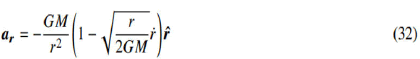
In this case, the second side must be zero to ensure that a force relationship between the stone and earth does not exist. Thus,

The initial vertical velocity of the stone should be equal to the escape velocity of earth’s surface which confirms our general knowledge and observations. Equation 32 can be written as follows:

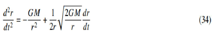
This second-order non-linear equation can be converted to an autonomous system in nondimensionalized and scaled form as follows:

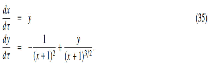
where x represents the distance of the stone from earth’s surface and y represents the stone vertical velocity. However, x(γ)=(γ(t)-γ₀)/γ₀ as x(0)=0 should not indicate the centre of earth but the surface of earth, whose radius is 1 unit. This system does not have a critical point and we will not seek equilibrium. Figure 5 shows the phase plane plot of this equation system.

As stated above the phase plane plots typically show the dy/dx slope at each point in the height-velocity (x,y) plane. The arrows in the diagram are the slope values at each point. If the arrow is horizontal, the velocity is constant and maintains its value. In the diagram, y>0 is the rise zone and y<0 is the free fall zone of the stone. The thick black line in the diagram represents the escape velocity. The value of the escape velocity is 1 unit on the ground surface in nondimensionalized and scaled formats and decreases by 1/√γ as it rises. In the y>0 region, the velocity increases where the arrow slope is positive and decreases where the slope is negative. The velocity change is slow at points where the slope is close to zero and faster at points where the slope is high. The velocity continuously increases in the y<0 region when approaching earth. The higher is the stone from the ground, the less is the change in speed [19].

If the velocity of the stone is greater than the escape velocity, its speed continues to increase but the rate of increase decreases as it moves away. In the region where the initial velocity of the stone is less than the escape velocity but near it, this initial velocity slightly decreases as it rises. But, due to the sharp decrease in the escape velocity, the stone upward velocity becomes larger than the escape velocity and starts to increase. The phase plane plots show that the repulsion effect (increase in the stone velocity) in certain conditions is part of the interaction. If the affected object does not have kinetic energy, it is completely under the control of the potential field and the field will pull it to the potential field intensive regions. As the affected body gains kinetic energy, it will become active in the interaction. If the kinetic energy of the affected object increases further during the interaction process while the potential field decreases, the potential field becomes repulsive. If the field potential energy and kinetic energy values are maintained, the equilibrium state will occur. In the interaction, the relative relationship between the field potential energy and the object kinetic energy (equivalently perceived velocity field) and the direction in which these components change during the interaction process are decisive. The interaction in nature is not only field relative but also dialectical as the effect of the interaction (form of change) also has a decisive role in the cause of the interaction (cause and effect dialectics).

Solution of the Flyby Anomaly

The flyby anomaly is an unexplained velocity increase that is observed when an object bypasses a gravitational source body at the shortest distance. This anomaly was first recognized after the earth flyby of the Galileo spacecraft in 1990; later, it turned out to be general (Edwards). Many different suggestions have been presented for the solution, but a consensus has not been achieved (Adler), (Iorio). The "Flyby Anomaly" creates a rather annoying situation for traditional physics. However, it can be said that, this problem almost exists to prove the correctness of the "field relative model of the universe" (Figure 5).

Figure 5: Interaction parameters of an object M2 as it passes through the vicinity of a velocity field source mass M₁.

Figure 6 depicts the passage of a spacecraft near a gravitational field source. The spacecraft flies in a straight line from A to C through B, which is the closest point to the gravitational field source mass. To simplify the calculation, we will assume that the spacecraft has a constant speed on its route. In this case, we will attempt to determine the acceleration that the spacecraft will expose along the route. For the spacecraft-mass interaction, we will neglect the spin velocity of the mass. In this case, from equation 18 for the spacecraft-mass interaction the perceived potential field will be:

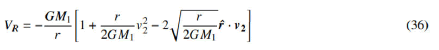
To simplify the calculations, we will assume the velocity of the aircraft along its route is constant and try to find out what its real acceleration at each point should be. This acceleration will have both radial and lateral components. The acceleration values are the values to be applied in opposite directions to maintain the spacecraft’s speed constant. Thus, the gravitational force that is applied to the spacecraft will be externally balanced and zero acceleration will ensure a constant spacecraft speed. Considering Figure 6 and assuming that O B is referenced horizontal axis, the term in equation 36, γ·ν₂=ν₂ cos α=ν₂ cos(π/2+φ) = ν₂ sin φ. Using these equations, the relative field potential (equation 36) can be written as follows:

Recall that the acceleration applied to the spacecraft will be the minus signed gradient of the relative potential field. After calculation, the following radial and azimuthal components of the acceleration are obtained:

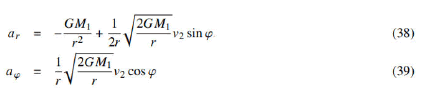
where φ is the lateral angle of the spacecraft on its route.

As the spacecraft moves from A to B, it will accelerate somewhat according to Newton’s law of gravity, as it will approach the source of gravity. However, as seen in equation 38, there is a second term in radial acceleration arising from the relative velocity field. Since the lateral angle varies from −φ to +φ, this second term will further increase the radial acceleration up to point B. Obviously, the increased radial acceleration further increases the orbital velocity as if the spacecraft were closer to the gravitational field source. Moreover, the spacecraft also has a lateral acceleration as in equation 39. This acceleration, like the second term in radial acceleration, is the product of the relative field velocity. The lateral acceleration will also increase the aircraft velocity up to point B due to both the γ−3/2 and the cos φ factors and then it will start to decrease. The second component of the radial acceleration becomes zero at point B then changes sign. That is, the second term of the radial acceleration will cause the spacecraft to slow down after point B.

Figure 6: Radial and lateral accelerations of a spacecraft during direct transition of a planet.

As the distance of point B to M1 is R=γ-3/2 cos φ, we can rewrite equations 38 and 39 as follow:

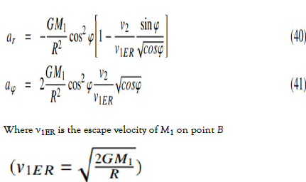
As it can be seen every parameter in Field Relative Model (FRM) can be expressed in terms of Newton gravitation multiplier. Figure 7 depicts the change in radial and azimuthal acceleration of field relative model as well as Newton gravity acceleration along the route in Figure 6. Obviously, accelerations in the FRM depend on the object velocity. In the Figure we assumed that the spacecraft travels along the route with the escape velocity at point B (v₂=v_1ER). The red track in figure shows Newton acceleration along the route having slightly higher acceleration at Point B due to the shorter distance to M₁. The radial acceleration component of the FRT causes the spacecraft to accelerate abruptly as soon as the transition process begins. This acceleration rate continues until point B, gradually decreasing. After this point, the speed of the spacecraft will begin to decrease. But the spacecraft is under the influence of FRM’s azimuthal acceleration too.

In the normal orbital route this component of acceleration depends on only the spin velocity of the source mass but, during direct transition of a planet the main source of velocity increase in the spacecraft is this azimuthal acceleration. As seen in Figure 7, the lateral acceleration will increase up to point B and then decrease. In the FRM analysis, geometric explanations are always our excellent assistants to visualize events with our mental perception. Accordingly, the basis of interaction in nature is related to how the affected object having a kinetic energy (velocity) perceives the potential field (velocity). In another words the perceived field velocity (i.e., "object velocity"-"field velocity") is the source of interaction force. Figure 8 shows the situation when the spacecraft bypasses the gravitational source mass. In the figure the red arrows represent the escape velocities along the route. The difference between the object velocity and escape velocities increases up to the shortest distance to source mass M1 then decreases. The change in this relative velocity causes change in perceived effective field velocity. The change in perceived field velocity is a function of both the distance to field source body and lateral angle. Therefore, its gradient both in radial and lateral directions are non-zero which cause both radial and azimuthal acceleration. The flyby anomaly is proof of the absolute accuracy of the field relative model of the universe [20].

Figure 7: Geometric explanation of Flyby Anomaly. The difference between the spacecraft velocity and escape velocities vary along the route causing perceived field potential to vary. This is the source of the Flyby Anomaly.

Figure 8: Interaction of binary stars. Each star will be attracted towards other star’s previous position.

Unstable interaction

So far we have considered the case when one of the interacting masses is very large relative to the other. In this case, the affected small object will see the field effect velocity of the larger one as infinite and equation 14 will be valid. However, when the mass sizes of the two affected bodies are equal or close to each other, the situation will be completely different. The situation is shown in Figure 9. Here M₁ and M₂ are interacting binary stars and orbit around the O centroid. In the figure, the mass of M₁ is greater than M₂, so the orbit of M₁ and its velocity are smaller. Let’s try to understand how they interact at a time t when mass M₁ is at point A and M₂ is at point B. Recall that the rates of interaction is finite and depend on the mass sizes in the field relativistic theory. In this case, the mass M₂ will be affected by the mass M₁ at point A₂ at time t₁ and the mass M₁ will be affected by the mass M₂ at point B₂ at time t₂. In other words, while the masses M₁ and M₂ are rotating around the center of gravity O, they will think that the masses acting on them are at the points B₂ and A₁, respectively. For this reason, the gradient of the relative potential fields (gravitational forces) is not towards each other, that is, neither of the masses will be under the influence of a central force. This explains why stars with similar mass sizes can never be stable. In this case, the relative velocity fields in equations 16 and 17 will be valid and none of them cannot be neglected. Since the escape velocities of the masses are dependent on their sizes, the t₁ and t₂ moments and accordingly the d₁ and d₂ distances will be different. If the masses are equal in size, the both time and distances will be equal and the two masses will rotate in their equal-sized orbits in positions exactly symmetrical with respect to their centers of gravity. It is seen that, in this condition, the relative velocity fields are time dependent. In other words, in order to calculate the interaction at a certain moment and at a certain point it is necessary to know at what time and where the source masses were in the past that formed current interaction force. The current force inter action depends on a distance and location in the past. We have to develop new solution techniques for these situations.

Field relativistic theory is universal. In other words, the theory is valid at the micro scale as well. Force field sources in atomic structure are close to each other in terms of both mass and electric charge sizes. Moreover, many source units are together and interact. Although the interaction distances are short, the speeds are quite high, so the spreading speed of the fields creates problems that cannot be neglected [21]. We think that this complex interrelationship lies behind the successful computation method developed with quantum mechanics, which not many people fully understand.

Conclusion

The field relative theory not only makes the solutions produced by the theory of general relativity easier to understand but also has the potential to create solutions for current astronomical and cosmological problems. This theory unifies all forces in nature and enables us to explore the micro and macro universe from a single perspective. In this article, the basic logic and mathematics of the theory and some applications in the macro universe are examined. Studies of the application of the theory to the micro universe are ongoing. However, readers will be able to easily understand the potential benefits of theory to entire physics by simply using the mathematics presented in this article:

The force interaction is not limited to gravitational attraction only, but the repulsive force is also part of the interaction according to the change in the object and field velocities in the interaction process. In the field relative universe model, there is another factor affecting the dynamics of two adjacent galaxies. Although not mentioned in this article, readers will easily notice that, if the spin axes of two adjacent spiral galaxies are in parallel and rotating in the same direction, the rotational field velocities in the region between the galaxies will be in the opposite direction and the resultant field velocity will be the difference (low velocity-high pressure zone), while in the external zones the velocities will be in the same direction and the resultant velocities will be summed up (high velocity-low pressure zone). Therefore, the spin effect of the adjacent galaxies will be repulsive under this condition. If the spin axes are in parallel but in the opposite direction, clearly the spin effect will be in attractive type.

Therefore, it is natural that galaxies approach and collide as much as they move away from each other. Consequently, the cosmological model presented by the field relative model is consistent with the observations. The expansion of the universe and the assumption of dark energy should be reassessed based on this notion.

The rotation of celestial bodies around their axes is not a coincidence but is a structural occurrence. The relative velocity field distribution within the volumetric celestial body causes it to rotate in a certain direction. Within the voluminous celestial body, if you move away from the effective field source, the rotational field velocity distribution decreases, while the linear orbital velocity of the parts constituting the affected object increases. Uncovering the rule of these spins using curl operation (Adams) in vector velocity field is an excellent practice of the theory.

In field relative interaction, the spin velocity of the source mass causes polar and azimuthal forces besides the central gravitational force. Investigating why all the planets in Solar system are not exactly on the same plane can be a good practice of theory.

Rotating celestial bodies create larger velocity fields on equatorial planes and consequently, denser energy fields. The higher is the rotational velocity of the source mass, the greater is the energy condensation at its equator plane. Therefore, the perceived mass of a rotating object at the equator plane is greater than its rest mass. Vigorous rotational velocities in celestial bodies are the source of flat clustering in nature. Any star, which is a member of a spiral galaxy, is under the influence the following field velocities:

• Both the escape velocity and the spin velocity fields of the rapidly rotating black hole in the center.
• Escape and trajectory velocity fields of all inner star clusters.

The total field velocity for a member star is the resultant of all the above velocity fields. We know that lateral field velocities lead to azimuthal acceleration as in equation 19 and Mercury orbital deflection is a product of this. Therefore, the orbital velocity of these stars must be substantially greater than Newton’s law of gravity foresees, i.e., field relative theory may not require the assumption of the dark matter.

Calculating the axis shift in Mercury would be another reasonable application of the theory. This application could not be performed in the study as the scaling factor k for the Sun must first be determined.

Light-mass interaction does not differ from mass-mass interaction where effective field is stationary. Therefore, the light changes its direction by being affected by the masses. The only difference about light is that its speed is the highest speed in nature. This extraordinary high speed causes a photon to be very slightly affected by the potential field because of two reasons:

• Due to the highest speed of the photon as an affected object, the escape velocity field of a source mass is hardly noticed, i.e., when νE<<c, then the perceived escape velocity by the photon ν=c-νE ≈ c ≈ constant. Recall that if the perceived field velocity is zero or constant, the object maintains its velocity. When the escape velocity approaches the light velocity, the light-mass interaction becomes evident. If the escape velocity source is a black hole, then only outside the event horizon νE ≤ c, therefore, light emission can only occur outside the event horizon.
• Due to the highest speed object velocity (photon), the interaction process is exceptionally short. The photon quickly moves away from the effective domain.

Traditional physics considers the speed of light is constant. In the field relative model, light is very slightly affected by the mass but not constant. For example, when light travels between the sun and earth at a constant speed, it travels approximately 500 seconds. According to field relative theory, as the photon is pushed away from the Sun, this time is 498 seconds on average. In the macro universe, the scaling factor is k ≪ 1 thus, the effect of spin motion in the interaction can be neglected, that is, the mass size is almost the only determinant in the interaction

In the micro universe, k is extremely larger than 1. Therefore, the dominant position of the mass size in the interaction has been replaced by the spin velocity. In atomic dimensions, the basic particles have very small masses but very high spin velocities. Therefore, the masses in the interaction can be neglected, i.e., even in the micro world, the field relative interaction is valid. The use of Newton’s universal gravitational constant G is indispensable in the force relationship in the micro universe. G determines the specification of the interaction medium in nature (space texture). Based on its dimension (m³/kg^·1/s²), G is a measure of both the thinness (inverse of density) and the flexibility of the space texture (ability to transmit velocity changes from one point to another point). Therefore, if a theory claims to be the theory of everything, it must use G in every scale. Readers must have realized what electricity is in our mental perception. Due to electricity, we have achieved scientific and technological development. Communication technologies have shrunk our world and nearly zeroed the process of access to information and space technologies have rendered almost every part of the universe observable. However, we still cannot define electricity. The new theory exposes that electricity is the spin velocity effect of particles. Details on this issue, for example, the + and - charges, the forms of attractive and repulsive interaction between them and how the two protons can pull each other although both have + charges are a separate article subject. Field relative theory can easily model all these problems.

Similarly, readers will notice that magnetism is also an effect of linear field velocity. This is why linearly moving charged particles (like an electric current flowing through a conductor) create a magnetic field. Because in this case there will also be a linear velocity component of the rotating field velocity (electrically charged particles). Since the space tissue behaves like an uncompressed fluid, the linear space velocity must somehow complete the cycle with cyclic motion. So there can never be a single pole magnet. In a magnet, the point where the linear field velocity starts and the point where it ends form two poles, while the field velocity from outside the magnet has to complete the cycle. Now readers will be able to easily visualize why two magnets attract or repel each other. How electrons must move through the magnetic material to produce a linear field velocity in a magnet is a very interesting and excellent instructive research topic.

The field relative interaction reduces all forces in nature to a single force: The gradient of the relative potential field caused by relative velocity field. The idea that such an interaction is valid in the atomic and subatomic universe is not clear to the scope of this article. However, we can understand it intuitively. Recall that on this scale, the rotational velocity fields (electric charges) instead of the mass form of the energy particles are dominant in the interaction. So almost the same interaction equation will apply. However, this time the mass size will be neglected and the spin speed with very large scaling factor will form the basis of the force. Here, readers will notice the feature that distinguishes the gravitational force from other natural forces. In the gravitational force, the resultant velocity of the field velocities formed by an infinite number of subatomic particles (escape velocity=energy dissipation velocity) is effective, while the field velocities of the subatomic particles themselves are effective in other forces.

Black holes do not have singularity (Einstein). When a massive star exhausts its fuel and starts to collapse on itself, the escape velocity approaches light speed, i.e., ν_E=c. In this case, the relative field velocity for all elementary particles that form an atom approaches light speed, i.e., ν_R=ν_p−ν_E=- c=constant. Recall that the constant perceived velocity field consists of the constant potential field and zero force field. Therefore, during the collapsing process of a star, the force relations between the elementary particles that form the atoms begin to disappear and the matter dissolves into pure velocity fields. A black hole is a pure velocity field and has no energy in substance form. An equivalent mass can be mentioned, but the bulk density and consequently singularity is meaningless. This equivalent mass can be found by Gaussian equation 5. The black hole formation process is the opposite process of the substance formation of energy particles and therefore, a process of entropy reduction locally. These topics are listed as new and exciting research topics that are immediately considered from the formulation of the field relative theory. The theory not only provides necessary solutions to the existing problems in physics but also creates different perspectives to better understand the universe.

Readers may think that the question "What is the escape velocity and its origin?" remains unaddressed. However, it may be estimated that this must be related to the tiniest element of existence in the universe. I present my solution proposal on this subject based on simple observations in my article titled "The Demise of Gravity Mystery" (Yalcin). Although some work has been performed during the development phase of the theory on these issues, these topics await the intense interest of scientists. The theory promises a more understandable universe as it considers that the workings of nature are more ordinary than previously thought. The theory is the updating form of Newton’s timehonoured theory with new knowledge and observations, which opens the door to a better understanding of nature. Another genius Einstein’s word is reaffirmed: "The most incomprehensible thing in nature is its intelligibility".

Acknowledgement

I would like to express my gratitude to Prof. Dr. Metin Arik and Prof. Dr. Birol Kilkis for their valuable recommendations, continuous support and encouragement. I am also grateful to Dr. Ariel Barton of the University of Arkansas for the web-based and user-friendly phase plane drawing program.

References

1. R Spiegel. Theoretical mechanics. Schaum Outline Series, McGraw Hill Book Company, New York, 1967, pp. 120.
2. Zee A. On gravity: A brief tour of a weighty subject. Princeton University Press; 2018, pp. 53.

   [Google Scholar]

3. Weinberg S. The search for unity: Notes for a history of quantum field theory. Daedalus. 1977;106:17-35.

   [Google Scholar]

4. Javid M, Brown PM. Field analysis and electromagnetics. Courier Dover Publications, 2019.

   [Google Scholar]

5. Moody MV, Paik HJ. Gauss’s law test of gravity at short range. Phy Rev Lett. 1993;70:1195.

   [Crossref] [Google Scholar] [PubMed]

6. Stewart J. Calculus. 8th Edition, 2015, pp. 1169.
7. Milgrom M. A modification of the Newtonian dynamics as a possible alternative to the hidden mass hypothesis. Astrophysl J, 1983;270:365-370.

   [Google Scholar]

8. Milgrom M. Mond theory. Canadian J Phy. 2014;93(2):107-118.

   [Google Scholar]

9. Batchelor GK. An introduction to fluid dynamics. Cambridge university press; 1967.

   [Google Scholar]

10. Spiegel, M. Schaum’s outline of theory and problems of theoretical mechanics: With an introduction to Lagrange’s equations and hamiltonian theory, 1967, pp. 33.
11. NASA. Studying the earth’s gravity from space: The gravity recovery and climate experiment. 2003.
12. Drinkwater, et al. ESA’s first core earth explorer, Proceedings of 3rd International GOCE User Workshop, 2007, 17, pp. 419-432.
13. Weisstein E. W. "Horn Torus." From mathworld–A wolfram web resource. 2019.
14. Jordan D, Smith P. Nonlinear ordinary differential equations: An introduction for scientists and engineers. OUP Oxford; 2007.

    [Google Scholar]

15. Sanchez Perez JF, Conesa M, Alhama I, Alhama F, Canovas M. Searching fundamental information in ordinary differential equations. Nondimensionalization technique. PloS One. 2017;12:e0185477.

    [Crossref] [Google Scholar] [PubMed]

16. Edwards C, Anderson J, Beyer P, Bhaskaran S, Border J, et al. Tracking Galileo at Earth-2 perigee using the tracking and data relay satellite system.

    [Google Scholar]

17. Adler SL. Can the flyby anomaly be attributed to earth-bound dark matter? Phy Rev D-Parti, Fiel, Gravitan Cosmol. 2009;79:023505.

    [Google Scholar]

18. Iorio L. The effect of general relativity on hyperbolic orbits and its application to the flyby anomaly. Sch Res Exch. 2009;2009(1):807695.

    [Google Scholar]

19. Adams RA, Essex C. Calculus. 8th Edition, 2013, pp. 912.
20. Einstein A. On a stationary system with spherical symmetry consisting of many gravitating masses. Ann Math. 1939;40(4):922-936.

    [Google Scholar]

21. Yalcin A. Demise of Gravity mystery. 2019.