Intro-The partitioned array data structure library and lineDB
Received: 25-Jan-2023, Manuscript No. PULJPAM-23-6101; Editor assigned: 27-Jan-2023, Pre QC No. PULJPAM-23-6101 (PQ); Reviewed: 10-Feb-2023 QC No. PULJPAM-23-6101; Revised: 21-Apr-2023, Manuscript No. PULJPAM-23-6101 (R); Published: 28-Apr-2023, DOI: 10.37012/2752-8081.23.7(4).1-5.
Citation: Duke Grable. Intro the partitioned array data structure library and lineDB. J Pure Appl Math 2023;7(5):1-5.
This open-access article is distributed under the terms of the Creative Commons Attribution Non-Commercial License (CC BY-NC) (http://creativecommons.org/licenses/by-nc/4.0/), which permits reuse, distribution and reproduction of the article, provided that the original work is properly cited and the reuse is restricted to noncommercial purposes. For commercial reuse, contact reprints@pulsus.com
Abstract
The partitioned array and now, the LineDB library aims to solve the problem of large arrays in high level settings. That is, they don’t work. Memory limitations and the limitations of hardware prevent an array database from storing, say, 1,000,000 entries. The partitioned array/ manager is designed to only look at a specific “file context" (and,”database” in ‘LineDB’), and partitions within that given ‘file context’.
While ‘LineDB’ resolves all problems of managing partitioned array file objects, it is still necessary to at least understand how to start a new object, allocate it, save all files to disk, get, and add elements to the object.
The ‘partitioned array library’ at its core, is capable of storing data created in the ‘partitioned array’ libraries to disk on function call. I found this very useful for anything, because now it is easy to manage an “array of hashes'” data structure. The file format it is stored to is the ‘JSON’ file format and object specification (‘javascript object notation’), and the partitioned array data structure uses the Ruby programming language, with ports for other languages such as ‘Rust’ and ‘Python’ on its way thanks to ongoing AI advancements..
Keywords
Partitioned; Ruby programming language; Analogy; Compost; Homeomorphic
Introduction
Class heirarchy tree
The class heirarchy is as follows, starting from the partitioned array and the class heirarchy has adecomposition, going down from the most abstracted to the managed/partitioned array. The managed partitioned array inherits from the partitioned array, and nothing else does. Variables are passed down the classes, even when starting from LineDB
Literature Review
The class heirarchy is as follows:
PAD=Partitioned Array Database
FCMPAM=File Context Partitioned Array Manager
FCMPA=File Context Partitioned Array
MPA=Managed Partitioned Array
PA=Partitioned Array
LineDB.PAD.FCMPAM.FCMPA (Managed partitioned array>partitioned array)# so called "class heirarchy (decomposition)";
Managed partitioned array
# inherits from partitioned array and thus partitioned array needs not be used over MPA.
Which is simply designed to give an overview of the approximate number of method nested calls one would have to do to use the managed partitioned array? Ultimately, every part of the data structure library uses the managed artitionedarray at the base level, and, even, according to the class hierarchy [1].
Data structures used
• Arrays
• Associated arrays/hashes.
• JSON/filename.json (Javascript object notation).
The fundamental data structures: “Managed' partitioned arrays”, …)
A “partitioned array” data structure (Synopsis)
The partitioned array’s fundamental characteristic is that all elements are placed into an invisible partition, meaning if you were to take out the data structure (‘@data_arr’), it would be a linear type of an array with a hash/ associated array in each indice, that is predictable and can be used apart from the classes used to create them.
Fundamental equation (non-algebraic) which defines a partitioned array’s “get” function:
# Special case; composing the array_id
if db_index.zero?
array_id = relative_id - db_index * @partition_amount_and_offset else
array_id = (relative_id - db_index * @partition_amount_and_offset)-1 end
A partitioned array is defined as a data structure which has “partitioned elements” within what should be a ‘regular array’
The data structure used for every element in the array is a Ruby Hash, or otherwise known as an associative array
Example of how a ‘partitioned array’ is structured, where each integer stands for an element index in the partitioned array (where a hash/associated array would be in place anyways):
‘Figure 69 (partitioned array structure):’
'((0,1,2), (3,4)..., (n, n+1))’
‘Caveat’: The first partition (‘(0,1,2)’ always contains the 0th element otherwise known as ‘0’ )
However, as a note: The partitioned array algorithm is currently coded in a way that it does not actually use subarrays; the algorithm takes responsibility for all aspects of the data structure (partitions, ranges, etc), so an array when defined by ‘fig 69’, would look slightly different, it would look like.
‘(0, 1, 2, 3, 4, n, n+1, n+2, ..., n+k)’
Note: The basic idea is you can store the array itself onto disk and “switch off” certain partitions, thus allowing for Ruby’s Garbage collector to take hold [2].
‘A partitioned array data structure works with JSON for disk storage, and a pure JSON parser is in progress. With two constants, the algorithm creates a data structure and allocates empty associative array elements and understands the structure of the partitions.’
The main purpose was I needed a way to divide an array into subelements, so that in gamedev I can flip on and off portions of the array in question to save on memory. The data structure overall is an ‘array of hashes’. For more information on the instance methods of the partitioned array, see the README.
Managed partitioned array (partitioned array specifications)
This will talk about the partitioned array and its suggested counterpart superset, the ‘managed partitioned array (lib/managed_partitioned_array.rb)’. In a great sense, the partitioned array could be considered the superset or fundamental basis of the data structure, going on out from the ‘partitioned array’.
The managed partitioned array adds a “file context” (database) to the partitioned array. It allows for the switching to a new “file context” on command.
This will do one thing: It will allow the programmer to switch to the new file context, in turn freeing up the memory of the previous partition or whichever partition the managed partitioned array was referencing. That is, it is a change of data structure “pointers” using “value objects” as the method of doing so (however, the LineDB database library fixes that).
A snippet of the table of constants (suggested variables that will be automatically used if you don’t specify in ‘object.new’).
# Db_size>partition_amount
Db_size=20 # caveat: The Db_size is the total # of partitions,
# but you subtract it by one since the first partition is 0, in code. # that is, it is from 0 to DB_size-1, but Db_size is then the max
allocated Db size
DB_MAX_CAPACITY = "data_arr_size"
DB_PARTITION_AMOUNT=9
DB_PARTITION_OFFSET=1
DB_PARTITION_ADDITION_AMOUNT=5
DB_NAME = "fcmpa_db" DB_PATH= "./DB/FCMPA_DB"
DB_HAS_CAPACITY = false DB_DYNAMICALLY_ALLOCATES=true
DB_ENDLESS_ADD = true DB_PARTITION_ARCHIVE_ID=0
# table of constants are used by default; check managed_partitioned_array.rb for usable constants, and the constants stated above
Mpa=mpa.new
# Switching to a new "file context" (db)
mpa=mpa.archive_and_new_db!
#Load a specific file context location (integer)
mpa.load_archive_no_auto_allocate!(file_context_location)
# load a given partition (partition_archive_id: Integer)
mpa=mpa.load_from_archive!(partition_archive_id: @max_partition_archive_id)
# Depends on the MPA variables, but will check to see if, the array is at capacity given
# that has_capacity is set
mpa.at_capacity?
# add a partition to the database; works with blocks:
mpa.add(return_added_element_id: true, and block) mpa.add do|hash|
hash("key1")="value1"
#..
end
# see PartitionedArray; returns a hash with additional data if set to true,
# and the id is the array element id
mpa.get(id, hash: false)
# in PA class, its load_all_from_files!
mpa.load_everything_from_files!
# in PA class, its save_all_to_files!
mpa.save_everything_to_files!
# an example of a low level variable
mpa.increment_max_partition_archive_id!
In order to use a managed partitioned array, you need to set a base directory and a few variable constants to set the database size and partitions (but they have default fallback values depending upon which library you focus on, as seen in the table of class inheritance constants).
Never ending array adds
MPA=ManagedPartitionedArray. New (endless_add: true, has_capacity: Fals e, dynamically_allocates: true) mpa.at_capacity? # has no use here
Finite length arrays
MPA=Managed partitioned array (max_capacity: "data_arr_size" (or some Integer), dynamically_allocates: false)
‘Use mpa.at_capacity?’ to detect when the array is full
Where max_capacity is the max number of array elements in a given partitioned array
Dynamic allocation
MPA=Managed partitioned array. new(dynamically_allocates: true)
##### Array split by file partitions (file contexts)
MPA=Managed Partitioned Array. new (max_capacity: data_arr_size,
db_size: DB_SIZE,
partition_amount_and_offset: Partition_amount+offset,
db_path: “ /db/sl", db_name: 'sl_slice')
# Where 'max_capacity' could be the max '@data_arr' size,
# or a defined integer.
# 'db_path' is the given folder that the database will
# reside in 'db_name' is the database's name
# Check if 'mpa.at_capacity?' to figure out if the MPA
# is at capacity (it returns true if at capacity)
# if it returns true, you can create a new file context:
Mpa=mpa.archive_and_new_db! # switch to a new file context (db)
Switching and allocating to a new file partition
MPA=Managed Partitioned Array. New (max_capacity: "data_arr_size",
db_size: DB_size, partition_amount_and_offset: Partition_amount +
offset,
db_path:"./db/sl",db_name:'sl_slice')
mpa=mpa.archive_and_new_db!
mpa.save_everything_to_files!
In the end if you need to load a new partitioned array, just specify it at the same given location and call ‘mpa=mpa.new’. This assumes that you are using the default constants, and if you want to do it explicitly, use ‘mpa=mpa.load_from_archive!’ and it will load from where it left off the last time the program was open [3].
File context partitioned array
This is an abstraction layer… It sets up the foundation for a database of partitioned arrays, but that is fully implemented as an abstraction in lineDB.
File context partitioned array manager
The file context partitioned array manager creates the database system for the partitioned array, but all it does is create managed partitioned arrays to create a database manager system for LineDB, which will be explained in lineDB below [4].
Discussion
Line database (linedb) the core library of the partitioned array
The line database is an abstraction layer class for the file context partitioned array manager (and the underlying databases), and the general uses of the partitioned array database will be covered [5].
Examples linedb/MPA diagram
Terse algorithm example: A terse example of the partitioned array’s get function, in which the rest of the algorithm uses as a basis, especially the equation [6].
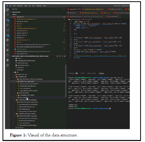
The algorithm uses ranges (inequalities in a sense, ex: 0..25) and I called the algorithm the ranged binary search (bsearch is the binary search in arrays), thus the algorithm’s search time for getting a given entry (extra overhead to, say, getting an array element straight from the array) is O (lg n). The weirdness derived from the equation is that in the 0th partition, there is always one extra element I call the 0th element, which means that in an ordinary partitioned array, there is always n+1 elements, where n alone is what the partitioned array would be in terms of its full element count (Figure 1) [7].
Intro the partitioned array data structure library and lineDB
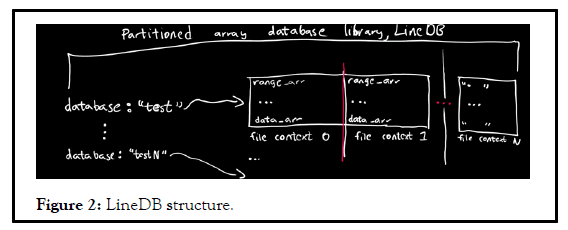
What has been stated before, is that the partitioned array is separated by partitions. This is true; the partitioned array when saving to disk saves it in variable chunks, and the range_arr dictates what partition one is looking at. This also means that you can load individual partitions of a partitioned array straight from disk, and you also do not need to load every partition at the same time. Algorithmically speaking, the managed partitioned array loads into the current file context. An example of how the partitioned array data structure looks in its abstracted class the LineDB will be placed below. In the code below, rel_arr and range_arr maintains the database’s structure, with rel_arr being the total number of elements in the partitioned array, and range_arr needed for the binary search in general. range_arr, is the number of partitions set to the partitioned array. In the case of for example, there are 3 partitions [8].
array_id’s final value would be the one to fit into data_arr to get the associated array data
# source:
https://github.com/ZeroPivot/partitioned_array/blob/master/examples/ range_bs_ex
# Ranged binary search, for use in CGMFS
# array_id = relative_id - db_num * (PARTITION_AMOUNT + 1)
# When checking and adding see if the index searched for in question
Partition_Amount=10
OFFSET=1
# When starting out with the database project itself, check to see if the requested id is a member of something like rel_arr
rel_arr=(0, 1, 2, 3, 4, 5, 6, 7, 8, 9, 10, 11, 12, 13, 14, 15, 16, 17, 18, 19, 20, 21, 22, 23, 24, 25, 26, 27, 28, 29, 30, 31, 32)
range_arr=(0..10, 11..21, 22..32) # in the field, the range array will have to be split according to the array, and the max id needs to match the last
range
puts range_arr
def range_db_get(range_arr, db_num)
range_arr(db_num)
end
db_index=nil
relative_id=nil
puts range_arr
range_arr.each_with_index do |range, index|
relative_id=range. bsearch {|element| rel_arr (element) >=33}
if relative_id
db_index=index
# we check to see if the relative id in the rel_arr matches the range
if range_db_get (range_arr, db_index).member? rel_arr(relative_id)
break # If so, then break out of this iteration
end
else
# If relative_id is nil, we don't have an entry at that location (aside from mismatching numbers)
db_index=nil
relative_id=nil
end
end
if relative_id
array_id=relative_id - db_index * (PARTITION_AMOUNT+OFFSET)
end
# relative id is nil if no element was found
p "DB number id (db_index): #{db_index}" if relative_id
p "The array database resides in (array_id): #{array_id}" if
relative_id
p "The array resulting value is (relative_id): #{relative_id}" if
relative_id
unless relative_id
puts 'The value could not be found'
end
# the implemented
LineDB example
b=LineDB.new(label_integer:true, label_ranges: true)
b("test").pad.new_table!(database_table: "test_table", database_name:
"test_database")
2000.times do |i|
b("test").pad("test_database", "test_table").add do |hash|
hash(:name)="name#{i}"
hash(:age)= i
end
end
In the example above, we create a new lineDB database and set it to b. Test was in the database text file and thus is loaded. The lineDB database takes a text file named textfile_fix.txt that has a line separated list of databases that are available. Upon startup, it should create the database structure [9].
b("test").Pad("test_database", "test_table") (0..25)
In this example, b calls the existing “test” database, then calls its partitioned array database, and the test table, which is a notation I added to the partitioned_array_database source code. Upon calling the Partitioned Array Database (PAD), we get the entries in the Database from 0 upto 25 [10].
Another example of class encapculation and inheritance decomposition:
# in: partitioned_array/decomposition.rb
require_relative "lib/line_db"
ldb = LineDB.new
p ldb.class #=> LineDB
zero = ldb("test") #partitioned array database
p zero. Class #=>partitioned array database b=ldb.db("test").pad
p b.class #=>file context partitioned array manager
p b.man_db.class\#=>file context managed partitioned array
c=b.man_db
p c.fcmpa_active_databases("_database_list_index").class\#=\>managed
partitioned array
LineDatabase=LineDB
PAD=Partitioned Array Database
FCMPAM=File Context Managed Partitioned Array Manager
MPA=Managed Partitioned Array
PA=Partitioned Array
Visual of the data structure
A visual is shown of the underlying data structure and use of the lineDB. “test” is the given database.
Using the lineDB.
The default searchup that LineDB seeks is a ‘db’ folder.
Place a ‘db_list.txt’ file into that folder with whichever number of databases you want, separated by line. In my case, I only created a database named “test”. mpa_text.rb is in the root folder of the partitioned array libr [11].
`require_relative
Quick note on getting LineDB working
Using git, do a git clone in the command line/terminal:
git clone https://github.com/ZeroPivot/partitioned_array.git
(Or download the release package on the partitioned array’s Github Page, named LineDB)
Into any given folder that you want.
Then, create a folder named 'db', and place in it a db_list.txtwith line separated database name of arbitrary choice.
require_relative "lib/line_db" or the location of the partitioned array library (lib) folder
There exists methods that add or remove databases (from db_list.txt) (Figure 2).
Some visuals of the data structure (Line DB)
Conclusion
The partitioned array is recent, and after a year’s worth of work I finally understand what I created, which was derived from a single equation and turned into an algorithm. If one needs extra clarification, e-mail me at EigenFruit@gmail.com, I have a lot of free time and I would be more than willing to assist. In the end the partitioned array is there to create a data structure in a specific way, and its aim was towards game engine development, but I also am using and testing it in a web development environment.
References
- Feschotte C, Pritham EJ. DNA transposons and the evolution of eukaryotic genomes. Annu Rev Genet. 2007;41:331-68.
[Crossref] [Google Sholar] [PubMed]
- Gayathri M, Shirasawa K, Varshney RK, et al. Development of AhMITE1 markers through genome wide analysis in peanut (Arachis hypogaea L.). BMC Res. 2018;11(1):1-6.
[Crossref] [Google Scholar] [PubMed]
- Gowda MV, Bhat RS, Motagi BN, et al. Association of high frequency origin of late leaf spot resistant mutants with AhMITE1 transposition in peanut. Plant Breed. 2010;129(5):567-9.
- Hake AA, Shirasawa K, Yadawad A, et al. Mapping of important taxonomic and productivity traits using genic and non-genic transposable element markers in peanut (Arachis hypogaea L). PLoS one. 2017;12(10): 0186113.
[Crossref] [Google Sholar] [PubMed]
- Kuang H, Padmanabhan C, Li F, et al. Identification of Miniature Inverted repeat Transposable Elements (MITEs) and biogenesis of their siRNAs in the Solanaceae: New functional implications for MITEs. Genome Res. 2009;19(1):42-56.
[Google Scholar] [PubMed]
- Lu C, Chen J, Zhang Y, et al. Miniature Inverted repeat Transposable Elements (MITEs) have been accumulated through amplification bursts and play important roles in gene expression and species diversity in Oryza sativa. Mol Biol Evol. 2012;29(3):1005-17.
- Makarevitch I, Waters AJ, West PT, et al. Transposable elements contribute to activation of maize genes in response to abiotic stress. PLoS Genetics. 2015;11(1):1004915.
- Mao H, Wang H, Liu S, et al. A transposable element in a NAC gene is associated with drought tolerance in maize seedlings. Nat Commun. 2015;6(1):8326.
[Crossref] [Google Scholar] [PubMed]
- Naito K, Zhang F, Tsukiyama T, et al. Unexpected consequences of a sudden and massive transposon amplification on rice gene expression. Nature. 2009;461(7267):1130-4.
[Crossref] [Google Scholar] [PubMed]
- Patel M, Jung S, Moore K, et al. High oleate peanut mutants result from a MITE insertion into the FAD2 gene. Theor Appl Genet. 2004; 108:1492-502.
[Crossref] [Google Scholar] [PubMed]
- Pfaffl MW. A new mathematical model for relative quantification in real time RT–PCR. Nucleic Acids Res. 2001;29(9):45.
[Crossref] [Googlesholar]


