Principles of Prime Numbers - Part II - Anatomy of Sppn & Rppn Tables with Conversion from mod10 to modNt Number System

Received: 04-May-2024, Manuscript No. puljpam-24-7133; Editor assigned: 05-May-2024, Pre QC No. puljpam-24-7133 (PQ); Accepted Date: Jun 19, 2024; Reviewed: 16-May-2024 QC No. puljpam-24-7133 (Q); Revised: 30-May-2024, Manuscript No. puljpam-24-7133 (R); Published: 30-Sep-2024, DOI: 10.37532/2752- 8081.24.8(4).01-12

Citation: McCanney J.M. Principles of prime numbers - Part II - Anatomy of Sppn & Rppn tables with conversion from mod10 to modNt number system. J Pure Appl Math. 2024; 8(5):01-12.

This open-access article is distributed under the terms of the Creative Commons Attribution Non-Commercial License (CC BY-NC) (http://creativecommons.org/licenses/by-nc/4.0/), which permits reuse, distribution and reproduction of the article, provided that the original work is properly cited and the reuse is restricted to noncommercial purposes. For commercial reuse, contact reprints@pulsus.com

Abstract

The prior paper “Principles of Prime Numbers - Part I - New Definition of Prime Numbers with ModNt Number System & Induction” must be read to put this paper into perspective. That paper is a summary of three books “Calculate Primes” (2007), “Principles of Prime Numbers – Volume I” (2010) and “Breaking RSA Codes” (2014). Another peer reviewed paper can be included in the list of prior papers “New Definition of Prime Numbers with Sppn Tables and Proofs by Induction”. In the prior books and papers, the concept of direct calculation of prime numbers was presented. It showed that the prime numbers constitute a complete number system modNt with a new visual representation in the form of “Sppn and Rppn Tables”. The understanding of Prime Numbers as a complete system of mathematics generated from Peano’s Postulates continues with visualizations of the results of using the “McCanney Generator Function” which directly calculates prime numbers in groups. The base N modulo number systems (e.g. the most common of which is mod10 or base 10) are shown to be inadequate to understand the true nature of Prime Numbers, which are the building blocks of all mathematics. It was shown that the mod10 or other base N number systems have been the hinderance to true understanding. The new modNt number system gives complete logical meaning to the prime numbers since every digit is related to the ancestry of the specific prime number showing them to have a unique “heritage” or “ancestry” back to the alpha prime 0 (zero). Many unexpected results arise on the order and properties of the prime numbers.

Key Words

Prime numbers; Number systems; Generator function; Nature’s number system

Introduction

This is part II of a multiple series set of papers building a completemathematical structure for the prime numbers, showing theyform a number system without the inclusion of other non-prime numbers. This and future papers will concentrate on the many details discovered by analyzing prime numbers as members of groups (they form a progression of groups with one generating the next) which gives rise to proofs by induction. This paper defines the structure of the Spp_n & Rpp_n Tables. It will also introduce the parameters that generate the next table from the prior table showing the nature of prime numbers from a completely different point of view [1].

Anatomy of Spp_n tables

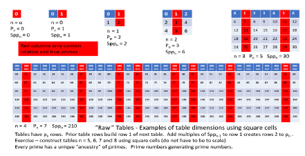
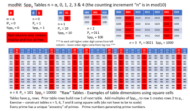
Spp_n means “the nth Sequential Prime Product”. It represents both the nth sequential prime product (product of all primes up to the nth prime) and is used to create the Spp_n Tables (with n incrementing from n = α, 0, 1, 2, 3 … ∞). The series of tables built below represent the visualization of the McCanney Generator Function (see prior papers referenced in the abstract). The sequence of tables is followed below by a generic Spp_n Table with some of the main features found in all tables. There are numerous forms of each table. The “raw” table has all numbers including non-primes with the “red columns” noted that eventually can be selected to create the “red only columns” tables (these uniquely contain all real and relative prime numbers). These can further be selected for “twin prime only tables” where only twin primes are managed in the given table. The “twin prime only tables” show that twin primes and only twin primes generate future twin primes as the tables are constructed from one to the next [2]. They can further be selected for other gap sizes or gap patterns. Each version has advantages depending on the problem one is trying to visualize. The “raw” all number table is useful in visualizing solutions to the Goldbach Conjecture, whereas the twin prime red column only table is essential in understanding the Twin Prime Conjecture. The full red column only table is best for understanding the symmetries of prime numbers, counting functions of prime numbers or sequences of higher order gaps (4, 6, 8 …) or gap patterns and the wave nature of prime numbers. Induction proofs are much easier to understand when visually enhanced. The tables below are first built with mod10 numbers and then followed by modNt numbers. The advantages of modNt numbers will become obvious whereas the limitations of mod 10 numbers will also become apparent. Tables n = α, 0, 1, 2, 3 & 4 follow (Figure 1).

Figure 1: Spp_n Tables n = ÃÂ?±, 0, 1, 2, 3 and 4 mod10

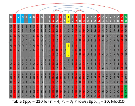
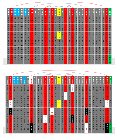
In above table Spp_n (n = 3) the twin primes occur in columns 1 and 5 (the origin and ancestors of all twin primes). They are (5, 7), (11, 13), (17, 19) and (29, 1). (23, 25) is not a pair that generates future twin primes because 25 (as shown in tables below) is not relatively prime to 30 = 2 x 3 x 5 since 25 has 5 as a factor. All future pairs of primes with gaps of 4 (using the definition of gap k_n = p_j – p_n) also originate in this table with n = 3. The table below is the same table but with red arcs over the twin prime pair columns including (29, 1). See part I paper for the explanation of this using group theory for closure. These tables form closed Groups and can further be reduced to just red column tables which contain only relative and real primes. They can further be reduced to having only twin prime red columns (where twin primes only are managed). Remember that relative primes are as much a prime as “real” primes in each table. Each table transforms in the progression of steps below where relative primes are identified in the table which will then generate the next table [3-6]. This may seem like a tedious effort, but it establishes the simple rules for creating future tables which become very large very quickly. It is the basis for solutions to unsolved problems using induction. The point is not to create large tables of prime numbers (although that is accomplished), but to create the mathematical structure to produce the induction proofs. Note that primes 2, 3 and 5 are colored with a light blue color showing that they are in the “Dead Zone” and will no longer generate future prime numbers (Figure 2).

Figure 2: Dead zone

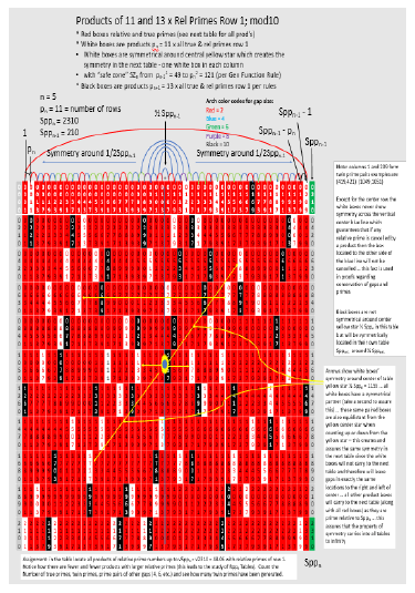
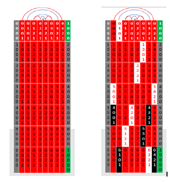
Below is the same table with white cells marked as products of pn = p4 = 7. They are symmetrical around the center point of the table ½Spp4 = 105. This is a fundamental property of all Spp_n tables. The white boxes are not relative prime to Spp4 = 210 = 2 x 3 x 5 x 7 because they have factors of 7, therefore they do not carry to build row 1 of the next table but all other cells including the black cells (products of 11 and 13) do carry over because they are relatively prime to 210. Since the white cells are symmetrical around the ½ point 105, this symmetry carries to the next table (symmetry is one of the basic properties of the Spp_n Tables and prime numbers in general). There is one and only one white box per column. The white cells are products of the red cells of row 1 with other red cells of row 1. These form a closed system so that when one eliminates the non-red cells, the red columns constitute a closed system containing only prime and relative prime numbers. In the future, the tables can be reduced to red column relative primes only (red columns) and further reduced to twin prime only tables (that generate only twin primes into all future tables). At this point one of the formulas for creating a new table from a prior table can be written. Since there is one white cell in each column, this constitutes the equivalent of a single row lost that does not carry to the create row 1 of the next table. So, the next table n = 5, Spp_n = 2310 for p_n = 11 row 1 will have 8 columns x (p_n – 1) rows = 8 x (7 – 1) = 48 cells symmetrical around 105 and 11 rows. The next table n = 6 will have 48 columns x (11 – 1) rows = 480 cells in row 1 symmetrical around 1155. This is the first of many equations that are developed to determine parameters of future tables without actually creating the tables, and thus forming the basis for proofs by induction. If you rotate the table with white cells only by 180 degrees, you see the same pattern of white cells showing symmetry (Figure 3). The black cells will exhibit symmetry when one arrives at the Spp_n tables for which they are p_n.

Figure 3: The black cells will exhibit symmetry when one arrives at the Spp_n tables for which they are p_n

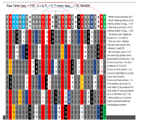
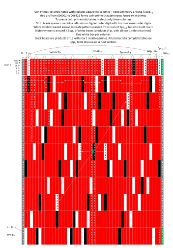
The following table is the same table with all products colored boxes. Read the notes to the side of the table. As the tables grow (faster than exponentially) it will become apparent that there will be a higher percentage of true primes, true twin primes and prime pairs of other gap sizes in each successive table. Try to look at the patterns of colored cells (first white, then black only, etc.) to see the patterns (noting that the tan boxes have multiple factors so are common to more than one pattern). This is to show that the products that eliminate cells from being primes can be generated without multiplying numbers. When only the red columns are isolated, the entire pattern of primes vs. relative primes is contained in the table (without a single calculation). When the modNt system of numbers is used farther below, the entire process will gain another level of simplicity since only the top row and left column cells need to be filled in.

When the rows are placed in sequence to form row 1 of the following n = 5 table with only the white cells not transferring, and since there is just one white cell in every row (making each row unique but symmetrical around the ½ point 105) these are the patterns that will shape the prime number patterns in the next table. These patterns are observed in the prime numbers and what have given rise to the belief that the primes are “pseudo random” when it is actually these patterns that are emerging. Part I paper defined “combs” and the wave nature of prime numbers. The combn is the series of relative primes of row 1 of the Spp_n table that repeats with wavelength Spp_n-1 to infinity with all primes predicted by this wave (in the form of an equation). Each successive table becomes more accurate at predicting primes. This gives rise to the rapid methods of breaking RSA codes and the accurate prediction of large primes (Figures 4 and 5).

Figure 4: This gives rise to the rapid methods of breaking RSA codes and the accurate prediction of large primes

Figure 5: The tedious part of this process is over except for one more table farther below that isolates the twin pimes only red column table

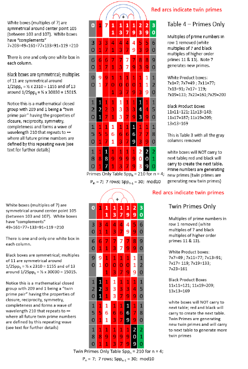
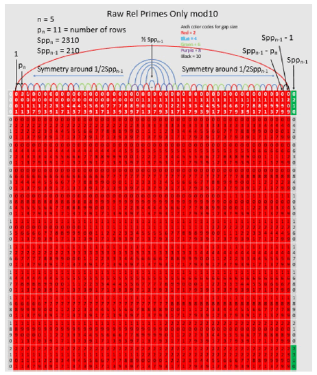
The following is the same table as those above but red columns only. This is done with each table creating the relative prime only tables. The tedious part of this process is over except for one more table farther below that isolates the twin pimes only red column table. Read the comments on the sides of this table. Each variation of the table (raw, red columns only or twin prime only) can generate the next table of the same type (raw, red columns only or twin prime only). Other variations exist such as gap = 4 or gap patterns but are not dealt with in this paper. In the side notes at the left of the table it notes that the black cells are symmetrical around the respective ½ points of the table when they are the current prime pn of that table. This could alternatively be constructed using the n = 4 table below by simply extending the same table down from the current table 11 times (210 x 11 = 2310 with ½ point 1155 for p_n = 11). Only the white cells are symmetrical around the ½ point of the n = 4 table and since these are the only cells that do not carry to create the next table, the symmetry carries to the next table. The pn prime p₄ = 7 where Spp_n – p_n = Spp₄ – p₄ = 210 – 7 = 203 are always white cells and therefore enter the Dead Zone DZ_n+1 of the n+1 table. This is a natural process that eliminates these numbers on each successive table increasing the size of the DZ on each successive table. The next table will have “1” in row 1 the first column and the next column as p_n+1 = p₅ = 11. On the right side of row 1 will have Spp_{n – 1} which is always a relative prime number (and sometimes a real prime, however it will always be relatively prime to Spp_n and will always carry to the next table to be symmetrical with 1 the top left corner cell). The next cell from the right in row 1 of the n+1 table will always be Spp_n – p_n to be symmetrical with p_n.

As with any of the tables, when looking at the table with white boxes only, if you rotate the table by 180 degrees, it will have the same pattern of white boxes (symmetry) and this then comes out in the creation of the next table. The twin prime only table above contains all the twin primes to this point (besides those lost in the DZ) but these are the ancestors of all twin primes (there are no others). The twin primes similarly form a compete number system without the aid of any other numbers. All future twin primes have one of these twin prime pairs as ancestors which in turn have ancestors in prior tables back to table n = 3. Pick any prime number or twin prime pair and as an exercise, find its ancestry back to this table (see paper Part I for more information on this process).

The next set of tables are for n = 5 mod 10. All the same variations are created as above ending in the twin prime only tables. This will complete the mod10 set of tables since it will be a rudimentary exercise to continue creating larger tables. The next steps will be to create the formulae that generate the parameters of future tables to begin the process of proofs by induction.

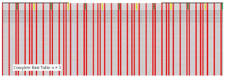
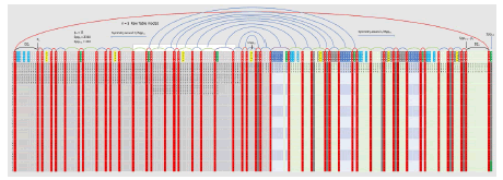
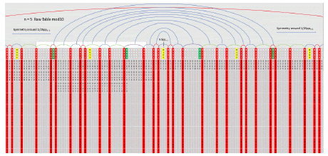
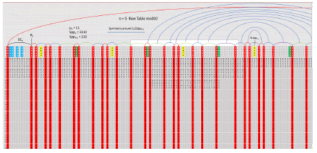
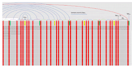
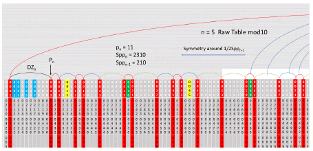
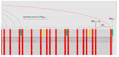
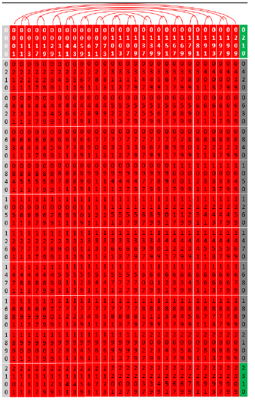
To generate the next table which is the raw table for n = 5, go to raw n = 4 table to generate the following raw n = 5 table. The table numbers are too small to see here so enlargements of portions of the table are listed farther below (Figures 6-12).

Figure 6: Raw n = 5 Spp_n Table - red columns contain all primes

Figure 7: Red arcs above adjacent red columns indicate twin primes and all other gaps are noted with arcs also. The end to end red arc is between column 1 on the left and column 209 on the right. The blue arcs represent symmetry of the patterns to the left and right of the center point 105 of row 1 (the blue arcs are not complete). See enlargements below for greater detail

Figure 8: Enlargement center region

Figure 9: Enlargement left region

Figure 10: Enlargement right region

Figure 11: Enlargement top left region

Figure 12: Enlargement top right region

Note in the above 2 diagrams that 7 and its complement 203 in row 1 have now moved into the Dead Zones (DZ5) between 1 and p₅ = 11 on the left side of the table and between 210 – 1 = 209 and 210 – 11 = 199 on the right side of the table (column p₄ = 7 and the column Spp₄ – p₄ = 210 – 7 = 203). This is a subtle but natural process resulting from the Generator Function and its single boundary condition. The following is the red column only table derived from the above raw table with arcs above the columns indicating the gaps between the columns (Figure 13).

Figure 13: Gaps between the columns

The following is the red only table with arcs above the columns and white cells (noting products of p₅ = 11) with one white cell in each column. The black cells are products of 13. To create row 1 of the following table for n = 6, use the rows of this table less the white cells stinging them together (and of course not using the 0 or 210 columns except for the very first cell = 0 and last cell = 2310). As an exercise, complete this table and see how many relative primes, real primes, relative twin primes, real twin primes, relative primes of gap = 4 and real primes of gap = 4 (Figure 14).

Figure 14: See how many relative primes, real primes, relative twin primes, real twin primes, relative primes of gap = 4 and real primes of gap = 4

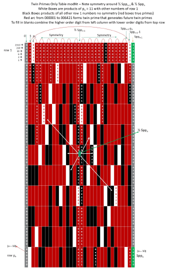
The following is the red column twin prime only table mod10 for n = 5 (this table not completed left for exercise but will be completed below for modNt case farther below). It is not a closed system in that the products of row 1 (unlike the complete red column table). The products of row 1 may or may not land in the table. There is a simple method of finding the white and black cell values in each column without the full table. Since there are two equations that exist for the numerical value each cell, the solution of these quickly gives the values of the cells that will be white (multiples of pn) and black (products of all other members of row 1 less than √Spp_n). The two equations for composite (non-prime) numbers are a) the product using numbers from row 1, and b) the top cell value plus a multiple of Spp_n-1. As twin prime only tables get larger, this is a simple method of determining real and relative primes (Figure 15).

Figure 15: The red column twin prime only table

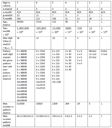
The following are the same tables but using the modNt number system. First there will be a quick review of the modNt number system before showing the modNt tables. For a more complete explanation review the paper Part I of this series. The following table gives the values of modNt vs. mod10 numbers up to 72 mod10. Note especially values of 1, 2, 6 and 30. These are the increments of digits in the modNt number system (as are 1, 10, 100 in the mod10 number system). Also note the values modNt for multiples of 30. Its usefulness will become apparent in the tables farther below. The limitations of the mod10 number system will also become apparent. Farther below is the formal definition of the modNt number system up to 510510 – 1 = 510509 (Figure 16).

Figure 16: modNt number system

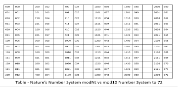
The following figures are the same tables as above but in modNt (see figure 17 below).

Figure 17: Numbers in each cell in the modNt number system

Determining the numbers in each cell in the modNt number system is easy (left column gives higher order digit and top row gives lower order digits (much simpler than mod10). To convert to mod10 simply multiply the digit by the value of the Spp_n for example the number from lower right-hand corner 006421 = 6 x 30 + 4 x 6 + 2 x 2 + 1 x 1 = 209 mod10. With modNt, you do not have to populate or write all the numbers since for any cell you can figure out the cell value by just combining the left column and top row. Note symmetry. With the same tables in modNt, the values of prime numbers can be easily determined without tedious long division nor multiplication and then easily converted to mod10.

See the patterns of the digits in the rows and columns with modNt numbers. Moving across in any given row the lower order digits follow the same pattern as row 1 numbers. Moving down in the columns only the higher order digits increment by 1. It is not necessary to write all the cell values because they are easily constructed with just the higher order digit from the left column and the lower order digits from the top row (Figure 18 below).

Figure 18: Higher order digit left column - lower order digits top cell

The following 2 tables are the red only table and the red only table with white cells (products of prime pn = 101 modNt = 7 mod10. These are then used to create the n = 5 tables farther below. It is left as an exercise to create the twin prime only red column table (Figure 19 below).

Figure 19: Red only table and the red only table with white cells

Below are the n = 5 tables in modNt number system. Note at the top left are the numbers with arrows 2310, 210, 30, 6, 2 and 1. These indicate the multipliers of the digits in the column for converting to mod10 and understanding the value of the digits in the numbers (3 tables build up to figure 20 farther below).

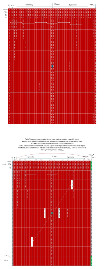
Figure 20: Only white cells do not carry to build row 1 of next table

Using the modNt number system, create the next table remembering that the white cells do not carry over. Also complete the multiples of all relative primes from row 1 and complete the black boxes. This will illustrate the processes and show how easy it is to produce the Rpp_n products (developed in the next section of this paper) and noting the issue with duplicate products using the raw tables (which include the red columns). Since the multiples of any relative primes form patters you can populate the tables with products without ever multiplying numbers as shown previously with the mod10 tables. The row 1 patterns are spaced (eg multiples of 11 or 13 or any other relative prime and remember to include all the relative primes). They form patterns and when you get to row 2 they fall in an offset but the same pattern all the way to row p_n. You will find that the rule for preventing duplicate products is that if the row 1 cell pj has a factor less than the number pi then it will create a duplicate product. The goal is to have the number of cancelled cells subtracted from Spp_n = number of real primes, or in the case of products of pn = the number of cells that carry to create the next table if you ignore the duplicate issue then you still will be left with all the real primes and without ever making a single multiplication.

Note the importance of √Spp_n as the largest element of row 1 that will produce a product less than Spp_n and fit inside the table and therefore the quotient (√Spp_n)/Spp_n-1 gives a value that becomes very small very fast. This gives a relative reading of the number of products of relative primes that will eliminate red cells from being real primes. There are more advanced modifications to this factor that will be more exact to show percentage more primes in each table, but just this factor is sufficient to show that the real primes, real twin primes, etc., will grow faster than exponentially in numbers with each successive table. It is the e = mc² equation of prime numbers. It is the key to understanding the large growth of prime numbers, twin primes, etc. using the modNt number system. Using the twin prime only tables, each successive table also has a “combn” equation that has a wavelength of Spp_n-1 that repeats to infinity just like the full red column tables, which then predicts all twin primes. Also as with the full red column tables, the accuracy becomes much better with every successive table. This has always been the difficulty with attempts at creating formulae for the discovery of prime numbers. They were limited in scope and rapidly broke down, producing more and more false prime solutions. This is now overcome in the current system. In the current system, the opposite is true as it becomes much more accurate with larger numbers.

The following table shows the twin prime only columns in red and all other columns in blue. Removing the blue columns creates the twin prime only table for n = 5, noting that the symmetry is maintained around both ½ Spp_n-1 = 105 (in row 1) and ½ Spp_n the center point of the table. As an exercise, pick an empty cell and determine its modNt value (using the left column and top row value) and then convert to mod10. The prime numbers are determined without division nor multiplication, but only using addition of the relative prime numbers of row 1 with the same multiples of Spp_n-1. In the third table below with red column twin prime only for n = 5 and white cells marked, you can generate the next twin prime only table for n = 6, however at this point the equations for generating the subsequent tables can be used without ever generating the tables (the following tables build up to figure 21 farther below).

Figure 21: The twin prime only n = 5 table

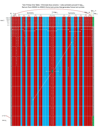
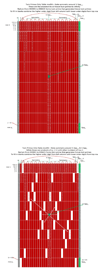
In the tables above, prime numbers form a complete isolated number system with Group properties of - closure – reciprocity – symmetry – completeness - and wave nature, starting with Peano’s Postulates and generating all prime numbers to infinity with each prime number having a unique ancestry back to the alpha prime 0.

Anatomy of Rpp_n tables

Rpp_n Table means “the nth Relative Prime Products Table”. The Spp_n Tables described above (with n incrementing from n = α, 0, 1, 2, 3 ... ∞) are generated starting with the n = α (alpha) prime 0 and Peano’s Postulates. When each Spp_n table is completed and the products of p_n x p_i (the white cells) are removed where pn is the nth prime number (associated with the nth Spp_n Table), and p_i = all relative primes of row 1 of the Spp_n Table, the remaining “cells” in the rows of the Spp_n Table are then used to generate row 1 of the next table Spp_n+1. There is one last step in working with the Spp_n Table before moving to the n+1 table. The step to complete table Spp_n is to determine the entire list of real prime numbers and gather parameters (for example: total number of real prime numbers, total number of twin primes, max gap values, value of (√Spp_n)/Spp_n-1, etc.) and then to create tables and graphs showing the progress as the tables grow. An appendix in Part I of this series gives an extensive list of parameters.

The values of relative prime numbers in the Rpp_n Table come from row 1 of the Spp_n Table as noted below. Recall in the prior papers that it was established that the relative primes in an Spp_n Table are as valid a prime number as “real” primes and therefore must be used in calculating the products that cancel cells (in discovering real primes). This is a very subtle aspect of the nature of prime numbers and the direct calculation of prime numbers. It is what has been overlooked prior to the current work. This is the key that unlocks the true nature of prime numbers and their ancestry. As noted in the prior papers, “Every Prime number has a unique history and ancestry going back to the alpha prime 0”. Some of the members of the ancestry may be relative prime numbers that as noted, are as real as “real” primes in a given Spp_n Table. These are composite numbers whose factors are prime numbers larger than pn and therefore are relatively prime to the sequential prime product Spp_n which has as factors all prime numbers up to and including pn. The unique ancestry of all prime numbers is seen in the modNt number that represents it. Additionally, each prime number has a family of related primes that were generated in the same “red column” and as such these primes are “siblings” and have “cousins” that were generated in adjacent columns in the same Spp_n Table. This also means that every twin prime pair has a unique ancestry as well as any other gap size or gap pattern. This conversely means that every twin prime (as well as relative twin prime pair) in each Spp_n Table will generate an infinite number of twin primes in future tables.

It is through the collection of parameters of the Spp_n & Rpp_n Tables (as they generate subsequent Tables) that begins the process of proofs by induction. Visual as well as mathematical understanding helps solidify the process just as geometric shapes help give visual confirmation of algebraic and trigonometric mathematics. The process of multiplying relative primes to locate real primes is a much more efficient process than using factorization division calculations to locate prime numbers since the prime numbers are generating future prime numbers. The goal is not to generate large tables of prime numbers (although this is a byproduct), but to create the parameters that will allow proofs by induction. The use of the modNt number system will facilitate the process since one does not have to fill in the numbers of every cell in the table, but only fill the top row and left hand column (these are used to generate the numbers in each cell making the entire process very fast). Any cell can easily be converted to mod10 numbers as will be shown. The tables become very large very quickly as noted in the prior papers. The Rpp_n Table shows the products that eliminate the relative prime numbers in the Spp_n Table, leaving only true prime numbers. There are simple rules to guide this process. Below the diagrams show a progression of Rpp_n Tables from n to n+1. A subtle issue is that there can be multiple products of relative primes from the Rpp_n Table that “cancel” a given “cell” so there are simple rules to prevent double counting the number of cancelled cells. Since the goal is to determine the number of real primes (the final count of cells that remain after all the relative prime products are calculated) this is not an issue.

One subtle feature of the products of any number from row 1 of a given red column only Spp_n table is that all the products of the given row 1 relative prime with any other number from row 1 results in a product that lies in the red column table. This means that each red column only table is closed (e.g. without the need for any other numbers). The prime number system is a closed system. This gives rise to the Rpp_n Tables (Figure 22).

Figure 22: Rpp_n Tables for n above and for both n and n+1 lower graph

The newly developed methods break the problems into pieces that can be solved individually then combined to give a complete solution. Previously, primes were thought of as “random or pseudorandom numbers with no patterns”. Trying to understand prime numbers as a linear progression has been partly at fault. Prime numbers are now organized and generate future prime numbers in groups and families with ancestors and descendants. This is key to creating the organization to solve more complex problems.

The “Calculate Primes” Generator Function system of directly calculating prime numbers is made more understandable in the current text because of the visualization using tables defined as “Spp_n and Rpp_n Tables”. It is the same prime number solution, but visual. By dividing the direct calculation of primes into small manageable groups which have well defined parameters and mathematical properties, one can now solve problems with understanding that was not available before. Each group generates the next group with known parameters giving rise to proofs by Induction. This is the “tool” that everyone has been looking for over the past 2500 years. The mathematical system, as explained in “Calculate Primes”, involves such mathematical properties as Closure, Symmetry, Reciprocity, Completeness and a wave pattern that allows equations to be generated with wave lengths that extend to infinity which become increasingly accurate with each successive table.

Finally, a system exists to predict the future of prime numbers and solves the issue of density of primes as one moves out on the number line. It is proven that the equations for prime number generation are simply bounded. The concept of finding “rogue primes” and “rogue gaps” is finally solved, and it is shown that in the Generator Function structure, prime numbers are a monotonically decreasing density function that is important in understanding prime patterns. Theorems are developed proving that all prime numbers generate an infinite number of future prime numbers and likewise all have ancestral patterns in the primes going back to the alpha prime “0”. These are used to understand and offer solutions to the Twin Prime Conjecture and Goldbach Conjecture unsolved problems. The prime numbers are generated in groups using the Generator Function by only addition and subtraction of previously discovered prime numbers (discovered in the prior iteration of the Generator Function) (Figure 23).

Figure 23: Sample generalized Spp_n Table

Generic Spp_n tables

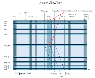
The example table above is a very simplified version of a generic Spp_n Table. This will be used as a basis for future papers to illustrate concepts. It may include symmetries for analysis of Goldbach pairs or it may be used to develop counting functions for twin primes. There are hundreds of variations of these tables showing different aspects of the primes with the list growing every day. Part of the usefulness is in understanding the subscript notation. There are many representations of prime numbers using the Spp_n and Rpp_n Tables and different ways of looking at the newly discovered sets of primes. The first is the rudimentary boundary condition where newly discovered real primes are all numbers pi such that p_n²in+1². These fall in the safe zone where there can be no composite numbers in the n+1 table. This is the natural process defined as the only boundary condition of the Generator Function. A second way of counting new real prime numbers is in rows 2 to p_n in each successive table using the Rpp_n Tables which find all real prime numbers in the table (without factorization).

There is another way of representing the numbers in Spp_n Tables. Since each number is locked in a grid of rows and columns and since each has a known set of factors (or is a true prime), these can be mapped onto a grid with mod10 integers and with a third number representing the lowest prime factor (p_min) of the cell (with 0 used to indicate a true prime). When discovering white cells of a given table to proceed with creating the next table (products of p_n with all other relative primes of row 1), and since there is symmetry around the ½ Spp_n value in the center of the table, one only must determine the white cells up to the center of the table since all the rest of the white cells are then found using symmetry. The 3 number representation (p_min , i_row , j_col) where i_row and j_col are the integer values of the row and column of the cell in the red column only table. With this information the entire Spp_n and Rpp_n Tables can be reconstructed but held with far less data than storing the entire set of numbers. The point of this Part II paper is to present the core ideas to understand the tables, but there remain many exercises for those interested in pursuing these leads. The point of this paper is to clarify the tables which lead to the proofs by induction.

Problem sets for Spp_n and Rpp_n tables

The following are examples of problems that can be solved using the information in Part I and Part II papers which give understanding to the order of the prime numbers as a complete autonomous number system. There are hundreds of similar problems that highlight the nature of prime numbers and eventually this series of papers will grow into a university level course complete with problem sets.

Calculate parameters of future Spp_n Tables and twin prime only tables.

• Determine the number of columns and rows (andtherefore the total number of red cells) in the next 3Spp_n Tables (for n = 6, 7 and 8). Do this without actuallycreating the tables. Note the number of cells in each rowof the prior table that will carry to form row 1 of thesubsequent table. Look for example in the n = 5 tablewith white cells and count the number of non-whitecells. You will count 43 cells in row 1, 44 cells in row 2,44 cells in row 3, 43 cells in row 4, 45 cells in row 5 and 42 cells row 6 containing ½ Spp₅. As you continue downthe rows these numbers will reverse since the table issymmetrical. The patterns of white cells will be exactlyreversed from the first rows (again due to symmetry ofthe table). Since there is only one white cell per column,all these patterns are different, and these sub patternscarry to the next and future tables. This constitutes anentire area of study.

• In doing so you will also be determining the number or“white cells” which are products of pn with all otherrelative primes of row 1 of the Spp_n Table.

• Determine the number of twin prime columns anddetermine the number of relative twin primes and realtwin primes in each table. These exercises will form thebasis for the solution to the twin prime conjecture. Onlythe white boxes do not carry to the following table. Notehow pn and (Spp_n – p_n) do not carry to the next table andenter the Dead Zone of the next table naturally. Theywill no longer generate prime numbers, although all ofthe relative primes that they generated (and theiroffspring) will continue to generate future prime numbers.

Using the symmetry of the Spp_n Tables to understand the GoldBach Conjecture

• Show why the Goldbach Conjecture local maximum valuesare located at Spp_n and multiples of Spp_n. This is a startingpoint to understanding the solution to the Goldbach Conjecture. Each real prime number in the red only tableshas a complement that is symmetrical around the centerpoint of the table ½ Spp_n which when added will be equalto Spp_n . Some of these pairs will have a relative prime that does not count in the final solution, however it maximizes the alignment of numbers causing the local maximums of GB pairs to be at Spp_n.

• Show that for all the solutions to the Goldbach Conjecturefound above (including if the numbers were relative primes), if you add or subtract 2 from either of the pairs ofnumbers to find a prime number (one of the GB pair ispart of a twin prime), then this produces a GB pair for Spp_n ± 2. There are other ways of using the tables toanalyze the GB Conjecture.

Deriving modNt numbers in Spp_n Tables and converting modNt numbers to mod10

• In any of the modNt tables above select an open cell ortwin prime set of cells and determine the modNtnumber(s)

• Convert this number to mod10

Determine the ancestry and future generation of a relative primes using the modNt numbers

• Using the same numbers as the prior exercise, determinethe ancestry of the modNt number(s) using the digits ofthe modNt number back to the alpha prime 0 (if a twin prime pair, also determine the original ancestor twin primepair in table n = 3; also noting that some of the ancestorsmay be relative primes in that table).

• Use any twin prime pair of row 1 of Spp₅ Table (n = 5) anddetermine the number of relative twin prime pairs thatcarry to the next table and then follow all of these to thefollowing table (noting that only the white cells do notcarry to the next table).

• 169 mod10 = 5301 modNt is a relative prime in tables n =4 and n = 5 since 13 is relatively prime in these tables.Determine the number of real prime numbers generatedby 169 before it enters the Dead Zone of Table n = 6,remembering that it still will generate relative and realprime numbers in table n = 6 where p₆ = 13. Thendetermine the ancestry of 169 back to the alpha prime 0(using the modNt number 5301) and convert to mod10numbers. Note that all the prime and relative primenumbers generated by 169 (its offspring and theiroffspring) will continue to generate prime numbers toinfinity. This leads to future discussion in future parts ofthis series dealing with the infinities of prime numbers(referring to concepts of Georg Cantor [6]).

Growth of primes, twin primes in future tables (counting functions)

• Since the size of the Spp_n Tables grows faster thanexponentially, the counting functions grow faster thanexponentially also. Look at the importance of the factor(√Spp_n)/Spp_n-1 and what this means on a given table. Theterm √Spp_n gives the upper limit of row 1 relative primeswhose square fits within the Spp_n Table. As the tablesbecome larger, this value rests farther to the left of row 1whose maximum value is Spp_n-1. So, this ratio gives anestimate of the percentage of products in the Rpp_n Tablecompared to the total number of red cells in the table.Since this number gets small very fast, it is the key tounderstanding the growth of the counting function whenviewed with Spp_n Tables. Since the tables grow faster thanexponentially, and since the traditional counting functionsare logarithmic, this gives a new method of understanding prime numbers. Rather than the prime numbers becoming fewer as you proceed out the lineal number line, they become more prolific.

• The combn equations predict all future prime numbers(derived from the list of relative primes of row 1 of table Spp_n) with wavelength = Spp_n-1 repeating to infinity topredict all future primes. Each successive combn predictswith greater accuracy and each comb reduces the numberof primes in the prediction (although the total number ofprimes increases because the wavelength grows). As aresult, there are no “rogue primes” or clusters of primes.This brings up the topic of density of primes. If there is alarge gap, then there will be an equalizing effect of manysmaller gaps in the vicinity and visa versa. As the primesgrow, the density of primes will become smoother (againthe result of only white cells transferring to construct thenext cell). This is a complex topic that requires analysisand is the topic of future parts of this paper.

Max Gap considerations (Max gaps do not carry to next tables only the evenly distributed pn products with relative primes in each table carry forward).

• Understanding of Max Gaps comes from the subtle aspectof white only cells of the Spp_n Tables. White cellsrepresent the products of pn with all other elements of row1 including 1. Since prime numbers generate future primenumbers, it might be considered that Max Gaps would alsocarry forward to affect future gaps. This is not the case.Since the white cells are the only cells that do not carryforward to form the next tables, and since the otherrelative primes (which cause the Max Gaps) do not carryforward, and since the white cells are evenly distributedthroughout the Spp_n Table, the Max Gaps do not carryforward to affect gaps in the future lists of primes.

• This also gives rise to the assurance that solutions to the Goldbach conjecture will not be affected by large gaps thatcould cause it to fail. These are advanced topics that will bepursued in future parts of this series.

Gap 4 prime pairs (the definition of gap in this paper is the gap k_n = p_j – p_i the difference between the two prime numbers)

• Since primes of gap 4 cannot be created from cancellingintermediate primes, they are like twin primes in that theonly prime pairs that can have gap = 4 are descendants oforiginal gap 4 primes (relative primes) in table Spp₃ with n= 3 (twin primes are separated by gaps of 4 so if one of thetwin primes is cancelled then it results in a gap of 6). Selectany gap 4 pair of primes and find their ancestry back totable n = 3.

• Use the same gap 4 pair of primes to determine all thefuture prime pairs of gap 4 (there will be an infinitenumber of them).

References

1. Principles of Prime Numbers - Part I - New Definition of Prime Numbers with ModNt Number System & Induction
2. McCanney JM. Calculate Primes with DVD Lecture, jmccanneyscience Press, Nashville, TN, 2007.
3. McCanney JM. Principles of Prime Numbers – Volume I,jmccanneyscience Press, Nashville. TN. 2010.
4. McCanney JM. Breaking RSA Codes, jmccanneyscience Press, Nashville, TN. 2014.
5. New Definition of Prime Numbers with Sppn Tables and Proofs by Induction
6. Contributions to the Founding of the Theory of Transfinite Numbers (Dover Books on Mathematics) by Georg Cantor