Principles of Prime Numbers - Part III - Sppn & Rppn Table Parameters with Advanced Topics and Twin Prime Conjecture

Received: 04-May-2024, Manuscript No. puljpam-24-7154; Editor assigned: 05-May-2024, Pre QC No. puljpam-24-7154 (PQ); Accepted Date: Sep 10, 2024; Reviewed: 16-May-2024 QC No. puljpam-24-7154 (Q); Revised: 30-May-2024, Manuscript No. puljpam-24-7154 (R); Published: 30-Sep-2024, DOI: 10.37532/2752- 8081.24.8(5).01-15

Citation: McCanney J. M. Principles of prime numbers - Part III - Sppn & Rppn table parameters with advanced topics and twin prime conjecture. J pure appl math.2024; 8(5):01-15

This open-access article is distributed under the terms of the Creative Commons Attribution Non-Commercial License (CC BY-NC) (http://creativecommons.org/licenses/by-nc/4.0/), which permits reuse, distribution and reproduction of the article, provided that the original work is properly cited and the reuse is restricted to noncommercial purposes. For commercial reuse, contact reprints@pulsus.com

Abstract

The prior papers “Principles of prime numbers - Part I - New definition of prime numbers with ModNt number system & induction” and “Principles of prime numbers - Part II - Anatomy of Sppn & Rppn tables with conversion from mod10 to modNt number system“ must be read to put this paper into perspective. Those papers are a summary of three books “calculate primes” (2007), “Principles of prime numbers – Volume I” (2010) and “breaking RSA codes” (2014). Another peer reviewed paper can be included in the list of prior papers “New definition of prime numbers with Sppn tables and proofs by induction”. In the prior books and papers, the concept of direct calculation of prime numbers was presented. It showed that the prime numbers constitute a complete number system modNt with a new visual representation in the form of “Sppn and Rppn tables”, creating the basis for proofs by induction for the twin prime conjecture and other problems.

Prior papers parts I and II presented many concepts with basic examples. The current paper part III expands on these providing more details and deals with the many parameters generated as the Sppn and Rppn tables progress to larger and larger sizes. Part I appendix listed many parameters associated with the tables (summarized in appendix 1 in this paper). Those values will be expanded upon. Most of these parameters can be represented in table or graphical form showing growth from one Sppn or Rppn table to the next and are instrumental in understanding the fundamental nature of prime numbers.

Key Words

Prime numbers; Prime conjecture; Graphs; Twin prime conjecture; Sequential prime product

Introduction

Prior paper details are expanded to show the complexity of the mathematical structure of prime numbers. Georg Cantor’s work of transfinite numbers is incorporated to show the different types of infinity when dealing with primes, twin primes and gap patterns. The question of whether there is an infinite number of twin primes has a more complex answer than just yes or no. Since the prime numbers are have ancestry from prior prime numbers in groups, and since the groups become more than exponentially larger in every Spp_n Table, the solution to the Twin Prime Conjecture is that “each twin prime generates an infinite number of subsequent twins”[1-7].

This is a different infinity than just a counting infinity as clarified in Cantor’s work. As noted previously, the view that the prime numbers lay on the linear number line is no longer a complete vista of the real situation. The idea that one would count the twin primes in sequence is not correct within the new definition of prime numbers. The prime numbers belong to groups and within these groups are family genealogies of the primes, twin primes and primes of all gap sizes and sequences of gaps. The prime numbers are generated in groups from prior groups and each prime, twin prime or other gap combination has an ancestry going back to the original prime, twin prime, etc. and all individual primes have an ancestry leading back to the alpha prime 0. This is a fundamental aspect of the McCanney Generator Function that presents the original simple definition of prime numbers with a single boundary condition. The following is a series of advanced topics building on prior Part I and Part II of this series.

Parameters of Spp_n tables – growth of Spp_n values

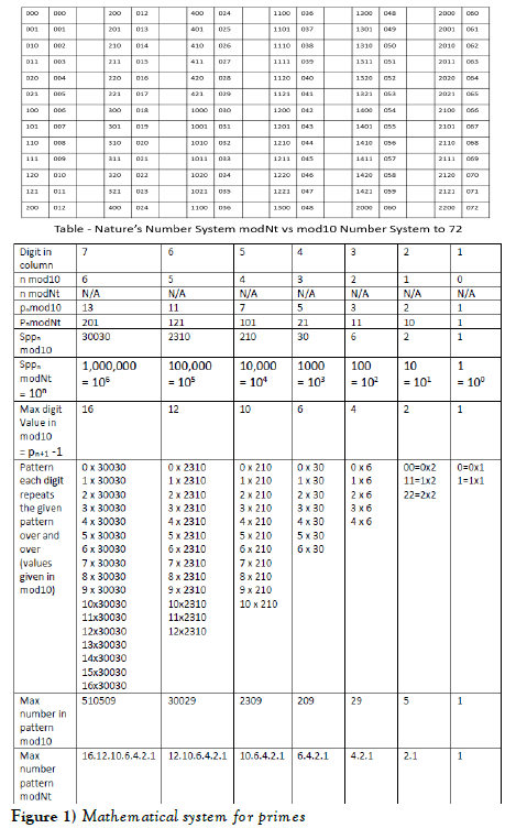
Spp_n means “Sequential Prime Product” and is the product of all prime number up to and including the prime number pn. In the modNt number system these are used to define each subsequent digit and represent the ancestry of the prime number back to the alpha prime 0. The modNt definition is reposted here for convenience of the reader. The conversion to mod10 is simple (multiply the modNt digit by the Spp_n value and add together). The modNt numbers when used in the Spp_n Table are easily discovered as they are made up of the higher order digit from the left column and the lower order digits from the top row. This means that to fill out all the numbers in the Spp_n Table only the top row and left column are needed, unlike mod10 numbers for which each number must be calculated separately. Even with mod10 numbers, the process of directly calculating prime numbers is faster and involves less computation than the traditional method of factorization to discover prime numbers. In addition to easily discovering prime numbers, it forms the basis for the complete mathematical system for primes. The following two tables are reposted from the prior Part I paper the values of mod10 vs modNt up to 72 and the subsequent table gives the definition of modNt numbers up to 510510 – 1.

The following two tables of values show growth of parameters with increasing values of the counting variable n of Spp_n tables. In Table 2 below some values are not given and are left as an exercise of those interested in understanding the patterns for total numbers of discovered primes and twin primes. The growth of discovery of primes and twin primes is more than exponential. This is the basis for upcoming proofs by induction for the prime and twin prime counting functions. Confidence is shown visually as well as mathematically that there is a more than exponential increase in solutions. Additionally, the fact that in the Spp_n tables only the white cells do not carry to form the next table is what has been missing from any prior analysis in predicting future outcomes. This is based on the new definition of primes using the McCanney Generator Function with the realization that relative primes in a given Spp_n Table are viewed as much as prime numbers as real primes. Future table parameters such as the size of the tables (number of columns and rows), the number of products of row 1 relative primes to “cancel” cells leaving real primes is essential to understanding.

Use the Spp_n tables from papers Part I & Part II to verify the above numbers. A few comments are in order regarding Tables 1 and 2 above. Regarding values in Table 1, the most important value is (√Spp_n)÷Spp_n-1 which becomes smaller with each increasing value of n the counting integer. This assures that the number of relative prime products of row 1 of any given table (which cancel potential prime numbers) becomes fewer proportionately in each successive table. In a prior paper this was termed the e=mc² of prime numbers. The end result is visible in Table 2 with the rapidly increasing values of “Total number of new primes discovered” with each successive Spp_n table. Physically, the √Spp_n value moves relatively farther and farther to the left of row 1 of successive Spp_n tables. In the Rpp_n representation of products of row 1, this means that the number of products that can “cancel” potential primes in a given Spp_n Table becomes less in every successive table, ensuring that the number of discovered true primes increases proportionately also. These observations, based on the new mathematical structure of prime numbers with the modNt number system and Spp_n tables, prove that the number of discovered real prime numbers (or twin primes) in each successive table is greater than the prior table.

In Table 1 the value of “Number columns red only table” for n = 11 is 1021870080. If the numbers in this red column only table were contained in cells of dimensions 1 cm x 1 cm, this would be 10218.70080 km long and with a height of 31 cm. Using another example with n = 8, the table for primes would be 0.92160 km long (about 921 meters) x 19 cm high. It would contain 603698 true primes and for twin primes only table there are 22275 column pairs so then there will be .22275 km x 2 (since these are column pairs) = .44550 km long = 445.50 meters long and 19 cm tall (p_n = 19) with 52817 twin primes identified in the table with no factorization performed. The rate of growth is more than exponential from one table to the subsequent table (Figure 1-9).

Figure 1: Mathematical system for primes

Figure 2: Cells leaving real primes

Figure 3: Complete raw table for n = 5

Figure 4: Enlargement top left region note DZ left side of table above

Figure 5: Enlargement top right region note DZ right side of table above

Figure 6: First review the Rpp_n

Figure 7: Example taken from table n = 5 using mod10 numbers

Figure 8: Horizontal white arrows indicate the divisions

Figure 9: Last two pairs have gap of 4 between them

In Table 2, the spaces between subsequent values of p_n² become larger faster than average gap size, thus, depending on difference between successive squares of primes, there will be more, or fewer primes discovered using the Generator Function Boundary Condition defined in paper Part I as p_n-1²in² but will generally be increasing.

In all cases where numbers of discovered primes are listed in Table 2, these values represent only the “new” primes found in the current table. To get the total number of primes up to the Spp_n value, add the value to all the prior values in the column to get the total number of primes discovered up to Spp_n. Note that these values are presumed to be exact, however, with such large numbers of entries it may be possible these numbers are not exact (if not exact they are very close to exact values). Their progression with more than exponential growth is notably correct and accurate.

Looking at the values in Table 2 for the “Number of column pairs for twin prime only tables”, they are calculated using the formula as follows. The values = the number of column pairs of the prior twin prime only table n-1 x (p_n-1 – 2) because there are 2 white cells of potential twin primes in every column pair. Since prime pairs differ by 2, if one member of a twin prime is a white cell, then the other member of the pair cannot be a white cell. The result is that there are 2 twin prime pairs lost to white cells in every twin prime pair of columns. Use the tables of Part I and Part II of this paper to count and verify this result. This is another example of an equation used to generate parameters moving from one table to the next. It also shows that the number of discovered twin primes grows faster than exponentially with increasing Spp_n tables.

The final values of some columns are left TBD.

Parameters of Spp_n Tables – DZ_n Dead Zones

DZn means “Dead Zone of the nth table” and represents the columns between 1 and pn on the left side of row 1 of table Spp_n and between Spp_n-1 -1 and Spp_n-1 – p_n on the right side of row 1 of table Spp_n (these 4 values are always relative prime to Spp_n-1 in row 1 of table Spp_n as explained in prior papers, however all the numbers in these spaces are not relatively prime). In these regions there can be no new prime number generation. This follows from the original definition of prime numbers in the McCanney Generator Function.

Essentially all numbers in this region are not relatively prime to Spp_n-1 and therefore when adding multiples of Spp_n-1 to create rows 2 to pn of table Spp_n, none of the numbers in these columns can be prime, thus the term Dead Zone with the counting integer n (DZ_n). In the diagrams (example below) the already discovered prime numbers to the left side of row 1 are marked in a light blue color, however the complimentary values on the right side of row 1 are never prime nor are any of their offspring in their respective columns.

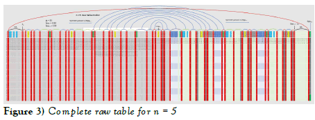
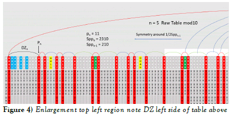
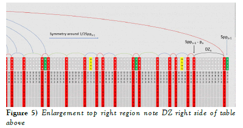
The following is reproduced from the Part II paper to illustrate the DZ₅ (n = 5 Spp_n Table). Note also the green cells in row 1 which are multiples of the prior Spp₃ = 30 table. Also marked in yellow are the midpoints of the comb for this table (values 15, 45, 75, 105, …) noting that 105 is the midpoint of row 1 of the current table. This illustrates that the prior table symmetries and structures carry over into all future tables. Combs will be discussed below but essentially the combn-1 is row 1 of this table and is derived from the complete set of relative primes that carry over from the prior table Spp_n-1. All members of the red columns are calculated adding multiples of Spp_n-1 to row 1 values. The following is the complete raw table for n = 5 with enlargements farther below.

Note in the above 2 diagrams that 7 and its complement 203 in row 1 have now moved into the Dead Zones (DZ₅) between 1 and p₅ = 11 on the left side of the table and between 210 – 1 = 209 and 210 – 11 = 199 on the right side of the table (column p₄ = 7 and column Spp₄ – p₄ = 210 – 7 = 203). This is a subtle but natural process resulting from the Generator Function and its single boundary condition.

The DZn creates a gap = pn – 1 = 11 – 1 = 10 on both sides of the table and for all values in their respective columns. These gaps are visible in the prime number tables. Pick any value of Spp_n in the prime number tables and go to the right (positive direction) and left (negative direction) and there will never be primes in these DZ_n Dead Zone regions. The same is true for all values of rows 2 to pn in the Dead Zone.

Below is a discussion of fertile equations for finding large primes and patterns of primes. Since 1 & pn and mSpp_n-1 ±1 & as well as mSpp_n-1 ± pn will always be relative primes to Spp_n-1 then these will be likely places to find large true primes. These will be much more productive than Mersenne searches and with the possibility of finding twin primes. The tables produce many other rich areas to find large primes, twin primes and primes of any gap or gap pattern. This also opens the field of not only finding large primes but finding all primes up to a certain value without factorization.

Parameters of Spp_n tables – Relative prime creates real twin primes

The relative prime 169 is part of a relative twin prime pair in Spp_n table for n = 4 (167,169). 167 is a real prime and 169 is a relative prime to the n = 4 as well as the following table for n = 5. It then appears in row 1 of Spp_n table n = 5 and is still relatively prime to Spp_n-1 = 210 in row 1 of table n = 5 (see table enlargement above) because 13 is relatively prime to 210. The point is that the relative twin prime pair (167,169) generates the following relative twin prime pairs in table n = 5, all of which will carry to the next table for n = 6 to generate more relative and real twin primes: (377,379), (587, 589*), (797,799*), (1007*,1009), (1217,1219*), (1427,1429), [skip (1627,1639) 1639 is a white cell with factor 11 and will not carry to the next table], (1847,1849*), [skip (2057,2059*) 2057 is a white cell with factor 11 and will not carry to the next table], (2267,2269). The * indicates relative prime but these will still carry to the next table to create more relative twin primes (that will carry to future tables) and of course more real twin primes. This is the fundamental realization that has been missing from the understanding of prime numbers and how they are created (this is contained inherently in the McCanney Generator Function). This leads to the result that every relative twin prime pair generates a downline and is ancestor to an infinite number of real twin primes.

Parameters of Spp_n tables – Why only one white cell per column?

One of the strangest results of the Spp_n Table structure is the fact that the products of pn with all other elements of row 1 of the table results in symmetrical distribution of white cells (cells no longer relatively prime) with one and only one in each column. Since the white cells are the only cells that do not carry to create the future table, the symmetry is also carried to the following table preserving the symmetry of the prime numbers in general. This begins with the n = α table and continues to infinity. The question is “why is there one and only one cell in each column of the Spp_n Table?

The answer is that the prime numbers form a closed number system completely independent of any other numbers outside of the Spp_n Table. Prime numbers have the properties of Closure (mathematical operations do not generate numbers outside of this system), Completeness (it is a complete number system in that all the prime numbers are discovered), Reciprocity (future tables are generated by prior tables and prior tables form an ancestry to future tables) and Symmetry (the Spp_n Tables possess many symmetries) and finally they have wave nature as explained by the “combn” equation structure with wavelengths repeating to infinity that define all prime numbers.

Regarding the white cells occurring one and only one in each column, the pn element of row 1 is multiplied by all elements of row 1 (including 1 and itself) so there are 48 products. It is in a sense stretching the row 1 values by a factor of pn with the final element value of row 1 multiplied by pn where Spp_n-1 x p_n = Spp_n. Another way of looking at this is that there are two equations that give rise to the cells of an Spp_n Table which are not prime. They are 1) the product pn x pj (all elements of row 1) and 2) the sum of the top row element and a multiple of Spp_n-1. Solving these two equations will result in one and only one value for each column resulting in one and only one value for each column.

Another interesting observation is that if you multiply pn with a pair of compliment relative primes of row 1 (symmetrical around ½ Spp_n-1 the half point of row 1 and whose sum is Spp_n-1), their respective products will create white cells symmetrically located around the center point of the Spp_n table with sum = Spp_n.

Parameters of Rpp_n tables

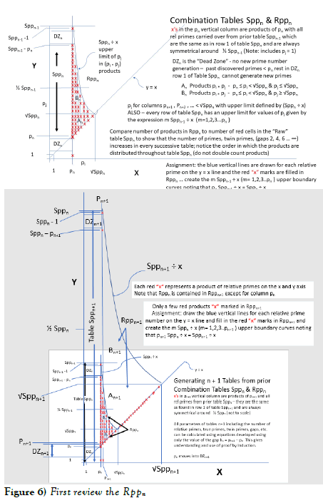
An Rpp_n Table is the summary of products of row 1 of a given table. These products cancel relative primes in the associated Spp_n Table leaving only true primes. This is accomplished without factorization and with minimal computation. The concept of Rpp_n tables was introduced in prior papers but needs more detailed explanations. Below is the progression of Rpp_n Tables from n to n + 1. Included are fine details such as the progression of pn into the Dead Zone of the next n + 1 table. The value of √Spp_n as an upper limit of row 1 relative primes that form products to “cancel” relative primes in the Spp_n Table is very important.

The “white cells” in an Spp_n Table are the products of pn with all other elements of row 1 of table Spp_n (including 1). Since p_n x Spp_n-1 = Spp_n, all products of pn with all members of row 1 (all of which are less than Spp_n-1) will fit inside the table. The prime number system is an autonomous system of numbers in that all these products fall in the red columns. There is one and only one product (white cell) in each column. First review the Rpp_n Tables below.

The White Cells are symmetrical around the ½ point in the Spp_n table (turning the Spp_n Table upside down shows the white cells in the exact same pattern and this symmetry carries all future tables). The following is a detailed guide for building the Rpp_n Table. It appears to be a lot of work on first glance, but the end goal is to understand the discovery of prime numbers from a viewpoint different from factorization which truly does require a great deal of computation. The goal is to develop generalized equations that allow analysis from a completely different perspective.

Take an example of a red cell only Spp_n Table with p_n contained in row 1. The red cell only table contains all prime numbers between pn and Spp_n. All prior primes less than p_n have already been retired into the Dead Zone DZ_n. The column containing pn continues to generate real prime numbers because it is relatively prime to Spp_n-1 since new primes are generated by adding multiples of Spp_n-1 to p_n so the pn column generates new prime numbers (this reverts back to the new definition of prime numbers and the McCanney Generator Function). The real prime numbers in the Spp_n Table are discovered by eliminating all the products in the table. The Rpp_n Table accomplishes this goal plus it creates an understanding with the most important aspect being the fraction (√Spp_n)/Spp_n-1.

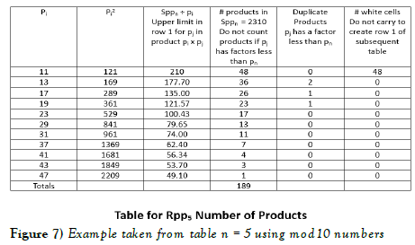
All products of relative primes p_i x p_j of row 1 of the Spp_n Table will fall in the columns of the table if and only if p_i < √Spp_n . There can be no products of any other rows that fall within the table. This is one of the amazing aspects of organizing the primes in the Spp_n tables. They are examined in bite size pieces. The Spp_n ÷ x curve of the Rppn Table sets the upper limit for p_j in the product p_i x p_j. Each prime p_i is tested to determine the largest relative prime of row 1 that will fit inside the table … p_j < (Spp_n ÷ p_i). In producing products of p_n p_n+1 p_n+2 … pmax where pmax < √Spp_n , since they have already been in products with smaller numbers of row 1, their products start at p_n² p_n+1² p_n+2² … p_max² . This leaves the lower end of the table relatively untouched by products whereas the upper regions of the tables have higher density of products. The following is an example taken from table n = 5 using mod10 numbers.

Note how the number of products reduces rapidly with increasing prime numbers. This is because the equation that governs the upper limit of the second factor Spp_n ÷ pi reduces rapidly. In the red column only Spp_n table for n = 5 there are 48 columns and p_n = 11 rows = 528 red cells. The Rpp_n table produces 189 composite numbers (see above table) so there are 339 real prime numbers of which 297 are new (rows 2 to p_n) compared to 36 in the prior table and 2903 in the following table. There are 480 relative prime cells = 48 x (p_n -1) that carry to form row 1 of the subsequent table n = 6. There are 15 twin prime column pairs (including columns 1 and 209) with p_n = 11 rows in the twin prime only table = 165 potential twin primes less 2 white cells in each column pair = 15 x (p_n – 2) = 15 x 9 = 135 relative twin prime pairs which carry forward to form row 1 of the n = 6 twin prime only Spp_n table (which will have p_n+1 = 13 rows). There are 55 new real twin prime pairs (rows 2 to 11) in table n = 5 (compared to 10 in the prior Spp_n Table and compared to 398 in the next table).

To prevent double counting of duplicate products (e.g. 13 x 121 = 1573 which was already counted in the white cells with 11 x 143), the rule is that in the product p_i x p_j if p_j has a factor strictly less than p_i then it will form a duplicate and do not count it in the Rpp_n Table. Duplicates first appear in the n = 5 table and become more prevalent in subsequent tables. This may seem like a complication, however when viewed from the use of the equation (√Spp_n)/Spp_n-1 these actually include the double counted products, so the actual fraction is less than that given by this simple equation. Another factor that makes this equation an upper limit is the fact that these do not account for the spaces between the prime numbers. The numerator term has an average larger spacing between primes than the denominator, making this fraction larger than it would be without this correction factor.

The region bounded by the vertical p_n line, the Spp_n ÷ x curve and the y = x line is divided into sections A_n and B_n. The An areas are similar triangles whereas the B_n areas become longer and relatively thin as you progress to larger values of the counting variable n.

There is a third dimensional aspect to the Rpp_n Table. Imagine that the product values be mapped in the Z axis for all products p_i x p_j produced, remembering that pn is multiplied by the entire row 1 including 1. Start at p_n² in the lower left corner of the An triangle and proceed to the pn x (Spp_n-1 – 1) product. Now imagine the entire field of products mapped in the Z dimension. This has applications in finding factors of numbers in the Spp_n Table since it can be used in reverse to find the factors of a given element of the Spp_n Table. There are applications that make use of this feature including finding factors of large numbers. This has applications in identifying RSA factors or simply finding factors of large primes in future tables to identify primality (a much less computational method than factorization).

The study of Rpp_n Table would take many papers to discuss all the properties related to the growth of the primes. It is the Rpp_n Table and its properties that give insight into understanding the more than exponential growth of the primes, twin primes and other gaps in subsequent Spp_n tables.

N = 6 Spp_n table and interacting waves built from prior tables

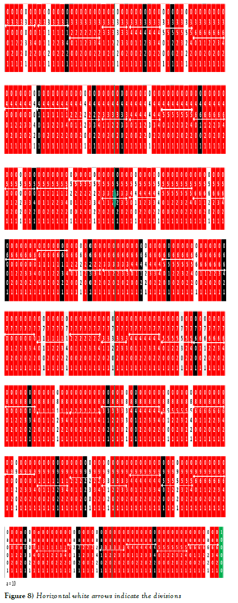
The following shows the wave patterns that carry from prior tables into future Spp_n Tables using the mapping of table n = 5 to n = 6 as an example. Part II of this series created tables up to n = 5 and left the creation of future tables as an exercise. Each table creates new wave patterns in the prime numbers which are not obvious, therefore this section is to illustrate these patterns. The unique symmetrical patterns arise from the fact that only white cells (relative prime products of pn with all other cell values of row 1 of a given Spp_n table) do not carry forward to create row 1 of the next (n + 1) table. Since there is one and only one white cell in each column of table n, the white cells of each row form a different and unique pattern. Additionally, these patterns are symmetrical around ½ Spp_n so that in the n + 1 table row 1 (created by putting the rows of the prior table in order), the symmetry carries forward into each new table. The patterns have been carried over from all prior tables and are imbedded in the tables. These patterns give the prime numbers their wavelike nature and is visible in the lists of prime numbers.

Previously, mathematicians stated that the primes appeared “as a random list of lottery numbers” or similar statements. If you pick any value of Spp_n or any of its multiples mSpp_n (m an integer) and look to the right and left of these numbers, for a short distance you see the patterns by adding and subtracting the relative primes of the Spp_n table in both the plus and negative directions (patterns of relative prime numbers). These patterns fade as other patterns emerge. Other effects such as the “conservation of prime gaps” show that if there is a relatively large gap, there will be many small gaps in the region to compensate. If there is a particularly small gap or series of small gaps (especially as the numbers get larger), there will be an equally large gap to compensate. This is a result of only white cells carrying to the next table to generate row 1. It is fundamental to see that the large or small gaps themselves do not carry forward, but only the evenly spaced symmetrical white cells. This states that large or small gaps or series of them do not affect the future patterns of primes.

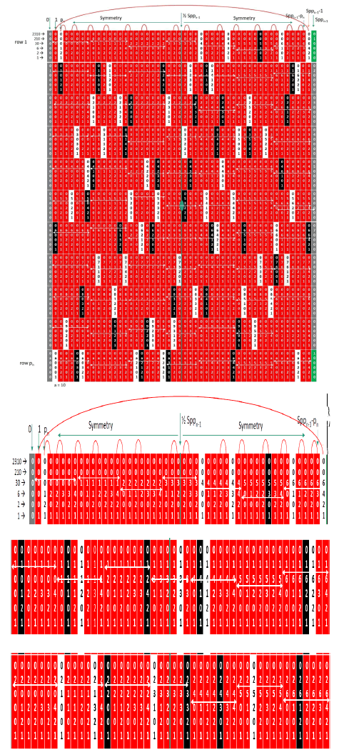
The following is the sequence of patterns that carry over from table n = 5 to create row 1 of table n = 6. String rows 1 through p_n = 11 together to create row 1 of table n = 6 leaving out the elements of 0 and 10000 columns (the first and last column). The numbers are modNt so it is an easy task to complete the numbers in every cell of the new table (using the left column value for the higher order digit and the top row value for the lower order digits). The first and last rows have an extra cell for 0 at the beginning and 100000 at the end to complete row 1 of table n = 6.

First the entire populated Spp_n Table for n = 5, Spp₅ = 2310 mod10 =100000 = 10⁵ modNt.

Horizontal white arrows indicate the divisions that carried over from table n = 4 with Spp_n = 30.

To complete the n = 6 table attach the above in a single string to create row 1 and then create rows 2 through p₆ = 13. The 0 column will have the following numbers listed vertically (modNt) with 7 digits in each number: 0000000 0100000 0200000 0300000 0400000 0500000 0600000 0700000 0800000 0900000 0a00000 0b00000 0c00000 where a, b and c are used in place of 10, 11 and 12 in modNt number system for convenience in the tables. To keep the table proportional, use 7 digits for all numbers in the entire table (using 0’s to fill space for smaller numbers).

The values in each cell of the table are easily constructed by using the value from the left most column for the high order digit and the top cell for the lower order digits. The white cells do not carry forward to create row 1 so you will eliminate the white cells before completing the table. The white cells are left in the above listing to show that the patterns in each row of white cells is unique, although there is symmetry around the ½ Spp_n value of 1155 mod10 = 53211 modNt noted in the above with a green oval dot. This symmetry carries to the following table and into all future tables. The goal is not to make larger and larger tables, but to build the mathematical system that will allow the general properties of primes to be studied from a theoretical point of view. Note also that the patterns that carry over from the n = 3 table (noted by the white horizontal arrows) are all unique on a repetition rate of 210.

After removing the white cells from the above pieces of row 1 of the n= 6 table, you will find that there are 48 – 5 white cells = 43 relative primes in the first one, 48 – 4 white cells in the second and so on. The final list of number of cells carrying to create row 1 of the table n = 6 will be in order: 43, 44, 44, 43, 45, 42 (where the ½ Spp5 center point is located), 45, 43, 44, 44, 43. From the center point out to the left and right, the numbers are in reverse order (they are symmetrical and also the patterns of white cells are in reverse order). If you take the first row and turn upside down it will show the same pattern of white cells as the last row. The second string if turned upside down will match the second to last, etc. This is physical result of the symmetry of table n = 5 which carries to the n = 6 table. This manifests itself in the white cells being symmetrical around the midpoint ½ Spp5. These patterns, like the pattern for 30 indicated by the white horizontal arrows, will carry into all future tables, giving the prime numbers their characteristic patterns. These are visible in the prime number tables if you know what to look for. Previously they were simply noted to be pseudorandom.

There is a fixation with prime numbers trying to see how many primes end in a certain digit or if certain modulo number systems favor a certain final digit, etc. A similar observation with mod10 numbers is that if the number ends with 0, 2, 4, 5, 6 or 8 then it is not prime. This leaves little to work with in the infinite set of prime numbers. In the modNt number system, to resolve the issue of the final digit, all of the prime numbers end in 1 so that solves that issue (although all odd numbers modNt likewise end in 1). The power of the modNt number system comes from the fact that all future primes will end in a pattern found in the tables above. If a number (no matter how large) does not end in a pattern observed in the above table, then it is not prime. This is true for all tables in modNt. As the tables get larger and the strings of digits get larger, the same rule applies that only if a number ends in one of the numbers in a given table could it be prime. The test would be to start with the smaller digits and work up to higher order digits. This would not be a practical method for determining primality, it is only interesting from the point of comparing this to old methods that did not reach this level of detail.

Comb_n-1 equations and the wave nature of prime numbers

Since the comb_n-1 equations predict all prime numbers to infinity in the form of a repeating wave of wavelength Spp_n-1, and since the equation for combn is built from the prior comb_n-1 by reducing the number of prime candidates, this defines the upper limit if prime numbers and creates a more exact prediction and creates a monotonically decreasing upper limit to all prime numbers. All future prime numbers are contained in this list. The comb definition is as follows. Comb_n-1 (note subscript = n-1) is the set of relative prime numbers of row 1 of table Spp_n (before removing multiples of p_n) carried from combining in sequence all rows of table Spp_{n-1 …} these are used to create the repeating wave of potential prime values to infinity. In general m Spp_n-1 ± comb_n-1 = pattern for all future primes (the patterns are symmetrical and extend to positive and negative infinity).

Where m is any positive or negative integer (although at present we only use the positive integers to predict positive primes). The generalized formula is combn-1 = (1, p_n , p_n+1 , … , Spp_n-1 – p_n+1 , Spp_n-1 – p_n , Spp_n-1 – 1) and forms a wave of wavelength Spp_n-1. The use of row 1 of table Spp_n was arbitrarily chosen (thus the use of the subscript n-1). All combs are symmetrical around the value of ½ Spp_n-1 which is visible in row 1 in the construction of the Spp_n tables. The comb_n-1 is an equivalent mapping of the Spp_n Table and is used to express the wave nature of prime numbers. The comb wave repeats to infinity and predicts all future prime numbers. There are applications in the areas of:

• Breaking RSA codes where all the prime numbers are not exactly identified but since one begins with the ability to calculate primes that can target specific regions of numbers, it makes it easy to quickly and simultaneously scan number pairs for size, high and low digit products to locate the prime factors, explained in detail in reference [5].

• Locating large prime numbers, twin primes and/or prime number patterns.

• Understanding the patterns found in prime number lists around Spp_n and mSpp_n values where m is an integer.

• In understanding the patterns found in Goldbach Conjecture pairs and relating solutions to future solution families (descendants and ancestors that are also GB solutions).

Examples using mod10 numbers:

m6 ± comb2 (n = 2 for Spp_n=6) where comb₂ = (1,5)

m30 ± comb3 (n = 3 for Spp_n = 30) comb₃ = (1,7,11,13,17,19,23,29) which are symmetrical around the ½ point of row 1 of table n = 4 which is 15.

Larger combs there will include all relative primes numbers (all true primes as well as all composite relative primes) that are relatively prime to Spp_n-1.

When the combs are written in modNt numbers, then the rule given in the above section applies. When looking for primality of very large numbers, if the number in question, when converted to modNt, does not have its final digits in the form of one of the members of a comb, then it is not prime. This is a far more powerful test than any previously given. It shows the power of the modNt number system in representing prime numbers.

Comb_n-1 equations and the wave nature of twin prime numbers

Twin prime only combn-1 equations are the same as all red table combn-1 equations but only including the row 1 numbers at the top of column pairs of twin primes. These likewise predict all prime numbers to infinity and with increasing accuracy as the tables get larger. Any other gap or gap pattern can be selected to predict future similar gap patterns with the caveat that for gaps of 6 or larger, new gaps of these sizes can be created as smaller gaps are eliminated by products of relative primes of row 1 with pn in table Spp_n which form the “white boxes” that do not carry forward to the next or future tables. This is an entire area of study only introduced in this paper.

One major point is that the twin primes and gaps of 4 form unique subsets of prime numbers because they are the smallest gaps and cannot be created in future tables by elimination due to white cells. All future prime pairs of gaps 2 and 4 will be descendants of the original prime pairs of table n = 3. These pair ancestries all revert back to table n = 3. There is a corollary regarding the “Conservation of Prime Gaps” which is an advanced topic. It states that once a gap is created, it will continue to generate into future tables to infinity. Again, this is due to the fact that only the white cells of a given Spp_n table do not carry forward to create row 1 of the following table, guaranteeing that some of the pairs in these columns will always carry forward and therefore will be found in future tables.

This is what has been missing from prime number analysis. Another fact of the process of directly calculating prime numbers is that the gaps never get smaller as the future tables progress, they can only grow larger. The gaps will always carry to future tables so will always occur in future tables and what is more, their locations are predictable. This removes the mystery of why small gaps (including twin primes) continue to occur even though the average gap size is very large. They are generated in a predictable manner by an infinite set of equations, each of which is a modification of the prior equation. Each successive equation removes possible prime candidates and thus creates a monotonically decreasing limit on primes, although the actual number of primes discovered by each subsequent equation grows more than exponentially. The limitations prevent what one might call “rogue primes” or “rogue gaps”. When an equation is constructed from row 1 relative primes and this combn-1 with wavelength Spp_n-1 is repeated to infinity, it defines all prime numbers (there can be no others). These form the properties of prime numbers of closure, completeness, reciprocity and symmetry along with the wave nature of the primes.

Safe zones and locating large primes and twin primes

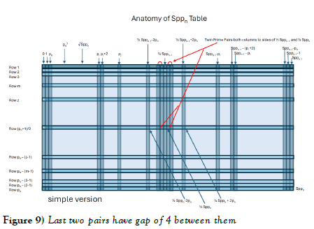
For many this will be one of the most interesting and important aspects of the new method of defining prime numbers. There are entire regions of the Spp_n Table that harbor what are called “Safe Zones”. They are twin prime pairs in adjacent columns that will always be relatively prime in their entirety (except for the single white cell in each column). Examples are the columns with top cell twin prime values of (1,(Spp_n-1 – 1)) which is the 1 column and Spp_n-1 – 1 column. They will always be relatively prime to Spp_n-1 and generate relative twin primes that will always carry to future tables to generate relative twin primes which will in turn generate real twin primes. To form the generated twin primes, use the prime from the (Spp_n-1 – 1) column as the first value of the twin prime and then use the next row value of column 1 for the second value of the twin prime. All examples of Spp_n tables in this series of papers show the red arc attaching these two columns indicating the generation of twin primes. Then there is the ever-present pair of twin primes

(( ½ Spp_n-1 – 4), ( ½ Spp_n-1 – 2)) to the left of ½ Spp_n-1

(( ½ Spp_n-1 + 2), ( ½ Spp_n-1 + 4)) to the right of ½ Spp_n-1 (the symmetrical compliment pair)

See the drawing below red arrows. These last two pairs have gap of 4 between them (which will always be there generating future gap 4 prime pairs to infinity). These are just 2 examples.

Also noted in the drawing above are the two cells to the right and left of ½ Spp_n in the center of the table with the following formula values.

p_n x ( ½ Spp_n-1 – 2) = ( ½ Spp_n – 2p_n ) to the left of ½ Spp_n

p_n x ( ½ Spp_n-1 + 2) = ( ½ Spp_n + 2p_n ) to the right of ½ Spp_n-1 (the symmetrical compliment)

These result from multiplying p_n with the row 1 elements adjacent to ½ Spp_n-1 the center point of row 1. These are significant because the region between ½ Spp_n and 2p_n to the right and left are “Safe Zones” that will never have white cells and therefore will always carry forward to form row 1 of the next table. So, there is a region of gap 4pn in the center of the table which will be a fertile location for finding primes. These are but a few examples of locations in the table that always carry forward with impunity. The reason that there can be no white cells in this area is because there are no relative primes between the values of ( ½ Spp_n-1 – 2) and ½ Spp_n-1 to form products with p_n therefore there can be no white cells in this area.

It has been pointed out previously and is contained in the McCanney Generator Function that in all tables, the values of 1 and (Spp_n – 1) will always be relatively prime and therefore will always be carried forward to generate future primes and more specifically twin primes. This gives another fertile area to search for large primes.

In addition to these, any relative prime, relative twin prime pair or pair with gap k or gap pattern has a chance of producing very large primes. These give much more fertile ground for searches such as GIMPS than Mersenne primes which offer a far lower return on computing investment. The current methods also offer the possibility that very large prime searches will produce prime pairs or other gap or gap patterns. A project in the background is a Spp_n computing system that will generate large tables of primes although with proofs by induction and the known prediction capabilities of the modNt number system, there is no longer the need for large table to test theoretical models.

Equation to predict number of red cells in prime & twin prime tables

If a given Spp_n table has column pairs (e.g. twin prime or pairs of gap 4, 6, etc.) which are first isolated into a table (e.g. twin prime only table), then, since each column contains one and only one white cell (relative prime not carrying to form row 1 of the future table) then the pair of columns will lose 2 pairs. The formula to predict the number of cells carrying to form row 1 of the subsequent table will be Mn (the number of cells in row 1 of the current table) multiplied by (p_n -2) = M_n x (p_n – 2). The generalized formula is

The following twin prime Spp_n table will have this number times (p_n+1 – 2) = M_n (p_n -2) (P_n+1 -2) and for the subsequent table M_n (p_n -2) (p_n+1 -2) (p_n+2 – 2) . The generalized formula for number of row 1 pairs of cells in a given table n = Z is given above.

The generalized formula for an Spp_n Table (counting single columns instead of pairs) is the same except replace 2 with 1 and replace Mn with the number of elements of row 1 of the current table. The table given in the section above entitled “Parameters of Spp_n Tables – Growth of Spp_n values” shows the numerical results for tables up to n = 11. The ability to determine the parameters of Spp_n and Rpp_n tables without actually building them shows another major value in this system.

Tables - alternate grid mapping of cells

The topic of the alternative Grid Mapping of cells was discussed briefly in the prior papers in this series. The Spp_n Table does not have to be filled in (because the cell values are constructed using the higher order digit from the left column and lower order digits from the top cell of the column). The entire table can be left empty, and any cell value can be calculated independently from any other. If additional future tables are needed in a particular study (as in breaking RSA Codes) then only the Rpp_n Table products need to be identified to create the subsequent tables. The Grid Mapping further reduces the data requirement. The advantage is far reduced data and processing to reach future tables where the data of interest lies. An alternative grid can be constructed with a triplet (x,y,z) number containing all the information needed to recreate the cell but with far less data and to generate future tables. The vertical left column is represented by the first number from 1 to pn giving the row number. The second number will be the column number of the red column only table. The third number will be the lowest prime factor and will be 0 if the number is a real prime (this number determined using the results of prior Rppn Tables). A further level of efficiency occurs because the white cells (products of pn with all other elements of row 1) are symmetrical around ½ Spp_n so only half of the white cells have to be evaluated, since the second half of the table is discovered using symmetry.

The amount of data is far less with the Grid Mapping method than if the cells contained the actual relative prime values especially as the numbers get very large. The third value of the triplet is used in counting the number of products of row 1 in the Spp_n Table. In creating the products from row 1 of p_i x p_j if the least factor of p_j is less than p_i then it will create a duplicate and therefore that product will not be counted. The third value of the triplet is lowest prime factor of the cell (set to 0 if the number is prime) and this is discovered in prior tables from the Rpp_n Table. This is an advanced topic requiring further publications.

Table uses - rapid identification of factors of large primes

If a number is contained in a red column only Spp_n table, then either it is a real prime or it has its smallest prime factor listed in row 1 of this table. This is major benefit of isolating relative primes (including real primes) in the Spp_n Tables. To emphasize this point, each Spp_n Table contains all true prime numbers between pn and Spp_n as well as relative primes (whose factors will always lie in row 1). Any number in row 2 or higher will not be factors of any number in this table. There are three reasons for making this statement.

1) any product involving a row 2 or higher number that would be less than Spp_n has already been eliminated in a prior table and

2) any product involving even the smallest element of row 1 (p_n) would be larger than Spp_n and therefore would not be in this Spp_n Table.

3) the red column only Spp_n tables are closed. Any number in the table that has factors will find those factors in row 1.

To identify factors of a number in a given Spp_n Table, use the Rpp_n Table Z dimension as discussed above in section “Parameters of Rpp_n Tables”. There are only a few elements of row 1 that are close to producing this value so it is relatively fast and easy to identify the lowest factor of the number. Coupled with the fact that one can produce Spp_n tables far into the future without completing all of the tables in between, produces a fast method for identifying factors.

Twin prime conjecture – proofs by induction

The three papers to date in this ongoing series have been building the basis for a solid proof of the Twin Prime Conjecture. Rather than viewing the numbers of twin primes as a diminishing set as you proceed to larger numbers (with anticipation that somewhere they will simply fade away), not only are the primes, twin primes, primes of gap 4 and other gap patterns seen to increase faster than exponentially in subsequent Spp_n Tables, but they increase because they are being generated by a known process. Their presence and location are predicted to infinity. The process is based on one Spp_n Table generating the subsequent Spp_n+1 Table with known properties based on equations. These start with Peano’s Postulates and only the number 0 the alpha prime, bridging between the most fundamental basis of pure mathematics and the prime numbers as a complete autonomous number system. The proof by induction has its basis firmly established. The next papers will complete the proofs in a formal way; however it should be clear at this point that the proof is complete and sound. There is an additional insight in that not only is there a solid proof for the Twin Prime Conjecture, but it states that every twin prime has an infinite number of descendent twin primes using the work by Georg Cantor on transfinite numbers. Not only does this method give a mathematical proof but also a visual representation that anyone can see. This is the understanding that has always been missing from analysis.

In addition to the twin prime conjecture, the basis has also been established for a new counting function for primes and other gap or gap patterns. The gap 4 prime pairs act exactly as the twin primes since, in the process of creating future Spp_n Tables, they cannot be created by eliminating intermediate relative primes as can happen with the other gaps. With this said, the gaps of any size that originate in a given Spp_n Table, although this is a subset of the entire group of gaps of this size, can serve as a basis for proving an infinite number of prime pairs of this or any gap size. This leads to the corollary “Conservation of Gaps” which is another topic that will be developed in future papers. It has far reaching implications in understanding prime patterns.

Goldbach conjecture - proofs by induction

Newly presented here are concepts that help in understanding the basis for Goldbach Conjecture solutions. It has been pointed out in prior papers that the reason there are local maximums of the Goldbach pairs at values of Spp_n (or multiples of these values) is because of the symmetry of the Spp_n Tables around the half point ½ Spp_n. The white cells eliminate relative primes symmetrically around the ½ point and therefore leaves all other red cells in the table. Every remaining red cell has a compliment cell that adds to Spp_n. The local maximums are a direct result of the symmetry of primes in the Spp_n Table. As you move away from Spp_n the “alignments” become fewer and many times the adjacent alignment creates far fewer Goldbach pairs. To find the number of Goldbach pairs for the number Spp_n – 2, combine all the prior solutions for Spp_n and find only those that are the second member of a twin prime pair. Combine these with the other number and their sum will be Spp_n – 2. To complete the process, take any two elements with real primes that add to a given even number and note their columns. In these columns there will be more prime pairs that add to that same number.

Looking at row 1 of the Spp_n Table, find two primes that add to an even number less than the max value in row 1 which is Spp_n-1. Follow the two primes moving down in their respective columns and the numbers generated in these columns are Goldbach solutions to the row 1 plus a multiple of Spp_n-1. This creates families of solutions just as the twin primes generate other twin primes. This is only introduced here and is a topic for one of the future papers in this series. The question is asked: “what would it take to break the Goldbach Conjecture”? This reverts back to the question of “conservation of gaps” with the caveat that for the GB Conjecture, the “gaps” may include real prime numbers between the gap end primes.

The riemann hypothesis – insights – proofs by induction

Work is proceeding in the background to map the Euler Equation into a form that can lead to proof by induction. It was imperative to release the current information up to this point. It has been made clear by others that the solution to the Riemann Hypothesis will not improve the ability to identify large primes. It is actually the contrary. If a large prime is discovered, it can map to a zero and not vice versa.

Problem sets for parameters of Spp_n & Rpp_n tables

The readers are encouraged to spend some time verifying the values and process given in this and the prior two papers and expand on the tables presented. It is only by going through the steps that the many unique aspects of this work can be appreciated.

References

1. McCanney JM. Principles of prime numbers - Part I-New definition of prime numbers with modNt number system & induction. J Pure Appl Math. 2024; 8(3):01-59.
2. McCanney J. Principles of Prime Numbers - Part II - Anatomy of Sppn & Rppn Tables with Conversion from mod10 to modNt Number System. . J pure appl math. 2024; 8(4):1-12.
3. McCanney JM. Calculate Primes with DVD Lecture, jmccanneyscience Press, Nashville, TN, 2007.
4. McCanney JM. Principles of Prime Numbers â?? Volume I, jmccanneyscience Press, Nashville. TN. 2010.
5. McCanney JM. Breaking RSA Codes, jmccanneyscience Press, Nashville, TN. 2014.
6. New Definition of Prime Numbers with Sppn Tables and Proofs by Induction.
7. Contributions to the Founding of the Theory of Transfinite Numbers (Dover Books on Mathematics) by Georg Cantor.