Specific case of an internal control-external control (bounded domain)

Received: 03-Sep-2024, Manuscript No. puljpam-24-7285; Editor assigned: 05-Sep-2024, Pre QC No. puljpam-24-7285(PQ); Accepted Date: Sep 25, 2024; Reviewed: 08-Sep-2024 QC No. puljpam-24-7285(Q); Revised: 13-Sep-2024, Manuscript No. puljpam-24-7285(R); Published: 30-Sep-2024, DOI: 10.37532/2752- 8081.24.8(5).01-03

Citation: Claver YP, Vuginshteyn A, Fuortes G, et al. Specific case of an internal control-external control (bounded domain). J Pure Appl Math.2024; 8(5):1-3

This open-access article is distributed under the terms of the Creative Commons Attribution Non-Commercial License (CC BY-NC) (http://creativecommons.org/licenses/by-nc/4.0/), which permits reuse, distribution and reproduction of the article, provided that the original work is properly cited and the reuse is restricted to noncommercial purposes. For commercial reuse, contact reprints@pulsus.com

Abstract

We try to study the controllability of bounded domain Ω consisting of several heated materials. For this, we will use the functional (μ), whichoptimizes the cost. The objective is to bring the excess heat inside the domain and also on the border of the domain and it’s this excess heat that is a function called control.

Key Words

Prime numbers; Prime conjecture; Graphs; Twin prime conjecture; Sequential prime product

Introduction

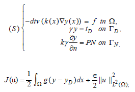
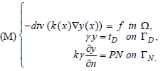
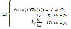
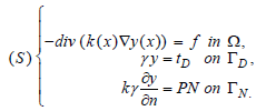
Let Ω be a bounded domain made up of heated materials, we give ourselves the conductivity (x) at the point x ∈ Ω the heat source ƒ in L^2(Ω) in the temperature T_D imposed on Γ_D by the system, the flux PN imposed on T_N. Let’s consider the following problem:

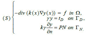
Problem

Let y_D be a given temperature.

How to act on the system (S) so that y is close enough to y_D?

Idea

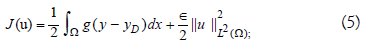
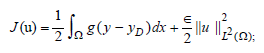
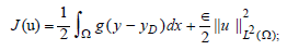
It is a question of bringing a surplus of heat u so that y is as close as possible to y_D [1-5]. This excess heat is a function called control [1-5]. To leave a good choice of u, we must optimize the cost, which reflects what we want to achieve and the means at our disposal. What amounts to considering the functional J(u) defined by:

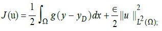
Where g is a definite function of Ω a value in â?. (y-y_D) makes is possible to minimize the difference between y and y_D, ∈ being very small serves not only to prove the existence and uniqueness of the solution but also to minimize the cost.

Problem

Is there Å« ∈ u such that

1. u is in the set of admissible controls,

2. Å« is the optimal control

3. y= y(Å«) is the optimal state

The function J is the objective function

However, there are two types of controls:

1. Internal control,

2. Border control

NB: we advise you to look at the course material on control for detailed proof.

Internal control

It is a question of bringing the excess heat inside the domain. Let us consider the following example of control:

Let ƒ in L^2(Ω), yD belonging to L^2(Ω) and u be a nonempty closed convex set of L^2(Ω) . Let u∈, (u) be the solution of the following equation.

Let’s pose

So we get the following problem:

Resolution

For any Z in L^2(Ω),we know the problem below

Has a unique solution in H¹₀Ω, therefore is the unique solution of problem (11).

We define the following operation:

Were Z is the solution of equation (4). A thus defined is linear and continuous.

We have

L^2(Ω),

By replacing (u) by its value in (2), we get:

Where

And is a constant.

Minimizing the functional J amounts to minimizing the functional J₁.

We put

1. a is bilinear,continous,coercive and symmetric,

2. l is continous linear,

3. u a nonempty closed convex set of L²(Ω),

By stampacchia’s theorem, there exists a unique Å« in u solution.

The solution Å« is characterized by:

Having obtained the existence and uniqueness of the solution, we are interested in giving the characteristics of Å«. To do this, we introduce the optimality system. By interpreting, the reaction

The Conjoint state is the solution of the following problem:

We therefore have

We get the following optimality system:

Particular case

In the case of shareholder internal Control, we have

Border control

This is to bring the excess heat to the Boundary of the domain.

Consider

The following boundary control example

Let ƒ in L²(Ω), y_D belong to L²(Ω), g a function of L²(T) and u nonempty closed convex of L²(T). Let u∈ u, y(u) be a solution of the following equation:

We pose:

Resolution

Simplification

By setting:

Where y₁(u) is the solution of the problem:

And z belongs to H¹₀(Ω) solution de :

System S₁ becomes

We pose:

Where

Transposition formula

We associate to (S₂) the following transposition equation:

Let ƒ be a function of L²(Ω) ( ) admitting a unique solution, we get from ( )

Considering the following problem:

l is linear and continuous application on L²(Ω) by riesz’s theorem, there exists a unique y ∈ L²(Ω) such that

We define the operator

Replacing

In J(u), We have:

With

We pose

Conclusion

In short, to solve the problem we must optimize the cost according to the goal we are looking for and taking into account the means at our disposal. But the case here requires a good mastery of the solutions of optimal control and some demonstrations to prove the existence, uniqueness and stability of solutions. Also, we give some extensions to our investigation.

References

1. Jormakka J. The error in the General Relativity Theory and its cosmological considerations. Preprint, 2024.

   [Google Scholar]

2. Jormakka J. On the field equation in gravitation. Preprint, 2024.

   [Google Scholar]

3. Jormakka J. On the field equation in gravitation, part 2. Preprint, 2024.

   [Google Scholar]

4. Jormakka J. The Essential Questions in Relativity Theory. Preprint, 2023.

   [Google Scholar]

5. Jormakka J. Failure of the geometrization principle and some cosmological considerations. Preprint, 2023.

   [Google Scholar]